Big Data - Plant gene expression workshop 1
Andrea Harper

Introduction
Aims
In this part of the workshop, we will look at some Brassica napus data. You are probably most familiar with B. napus as bright yellow fields of oilseed rape, but the species also includes the vegetable swede, some exotic varieties grown in places like China, and fodder crops for cattle. The complete dataset includes three files, a large dataset of gene expression data for 101 different lines of B. napus, a file with the content of glucosinolates in the seed oil for each line, and a file with information about where each gene is in the B. napus genome. For this workshop, we will work on a smaller expression dataset, but you can find the complete one you will need to complete a full analysis here, or from the Data Sets tab in the VLE.
Learning Outcomes
By doing this practical and carrying out the independent study the successful student will be able to:
- open and explore large gene expression datasets
- clean up and subset datasets as required for gene expression analysis
Getting started
The words ‘folder’ and ‘directory’ mean the same thing (for most purposes). Folder is mainly a Windows term; directory is more classical and widespread.
I like to work in one folder named for the particular task. I recommend creating a folder called Big Data (or similar) containing folders called ‘data’ and ‘scripts’.
Start RStudio from the Start menu
In RStudio, set your working directory to your scripts folder
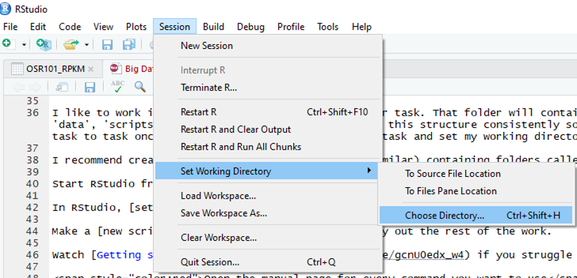
Make a new script file to carry out the rest of the work.
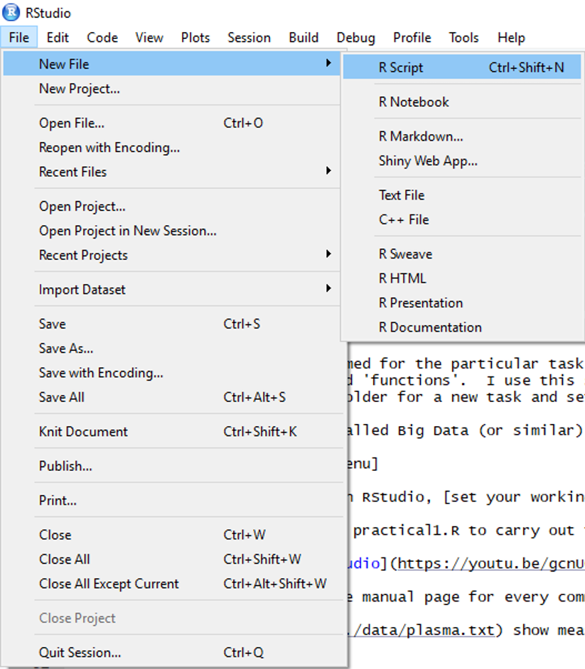
Open the manual page for every command you want to use
The data in OSR101_sample.txt show measurements of gene expression in a random sample of 101 Brassica napus (oilseed rape) cultivars. The gene expression measure used here is RPKM, or reads per kilobase per million aligned reads.
Read the sample data file into R
OSR101_RPKM <- read.delim("http://www-users.york.ac.uk/~ah1309/BigData/data/OSR101_sample.txt") You should find a view of the data appears and an object called OSR101_sample can be seen in the Environment window. If you are having difficulty, Reading in data files might help.
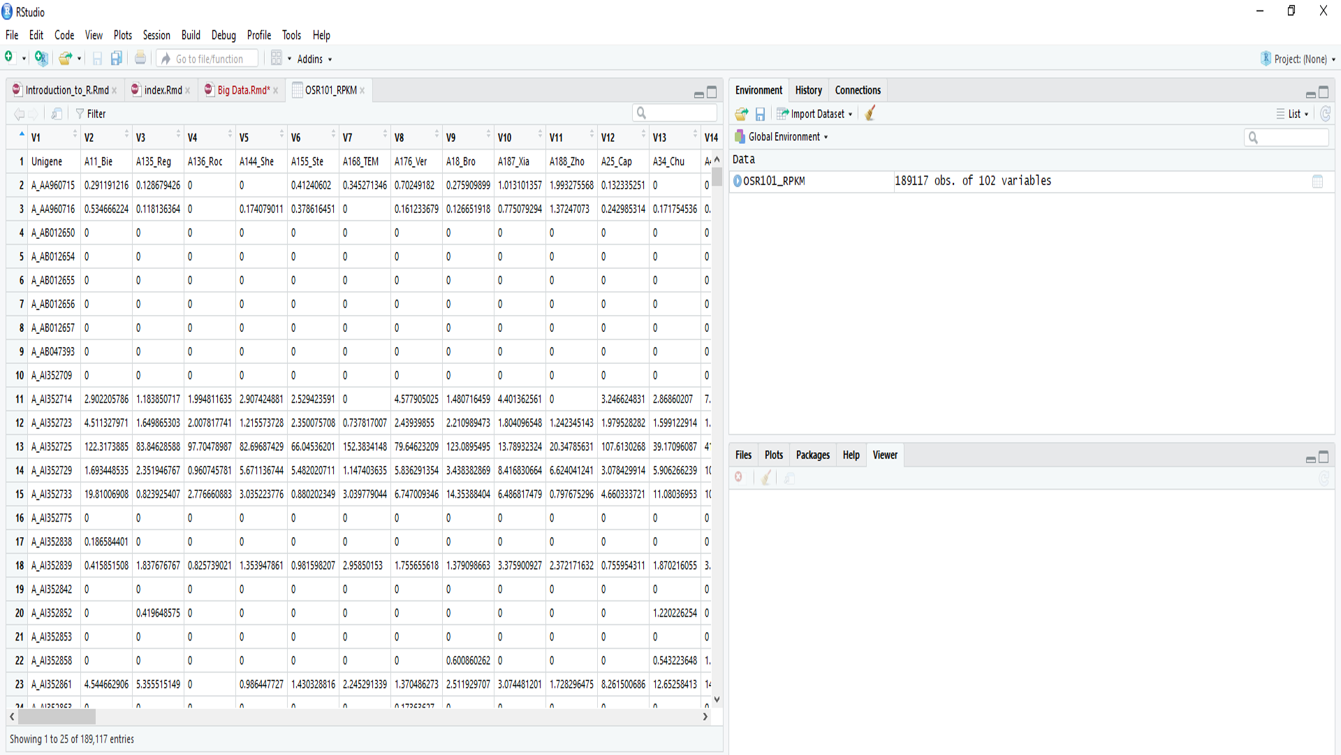
What is the biological question?
Using this data, we would like to know which genes are involved in changing the level of glucosinolates found in the seed oil. If you want to know why glucosinolates are important, take a look here
Get to know your data
Use class(OSR101_sample) to see what type of data you have, and dim(OSR101_sample) to see how large it is.
class(OSR101_RPKM)## [1] "data.frame"dim(OSR101_RPKM)## [1] 100 102It looks like the file is a data frame (contains both numbers and text), and has 100 rows, and 102 columns.
You can tell R which rows and columns you are interested in using square brackets. Rows are always the first number and columns the second, and they are seperated by a comma. If you want all rows or columns, don’t put any number.
So, let’s take a look at the first 5 rows and 6 columns of the data…
OSR101_RPKM[1:5,1:6]## Gene A11_Bie A135_Reg A136_Roc A144_She A155_Ste
## 1 A_JCVI_10003 5.59343127 2.57476690 2.4295783 3.794030 7.92182114
## 2 A_JCVI_10016 1.26169112 0.07965001 1.6105420 0.000000 0.00000000
## 3 A_JCVI_10018 10.61947131 7.44378077 8.9981791 4.292112 8.90302512
## 4 A_JCVI_10019 2.07634949 2.09726467 2.7240726 1.931506 2.38054726
## 5 A_JCVI_1002 0.07684213 0.13582828 0.0762911 0.000000 0.07255291Or the first 2 rows and all columns…
OSR101_RPKM[1:2,]## Gene A11_Bie A135_Reg A136_Roc A144_She A155_Ste A168_TEM
## 1 A_JCVI_10003 5.593431 2.57476690 2.429578 3.79403 7.921821 4.2833250
## 2 A_JCVI_10016 1.261691 0.07965001 1.610542 0.00000 0.000000 0.4274322
## A176_Ver A18_Bro A187_Xia A188_Zho A25_Cap A34_Chu A42_Dar A87_Les
## 1 5.622508 6.735284 3.648835 1.994188 6.143167 8.3851445 5.622014 3.122881
## 2 1.087071 0.000000 0.000000 0.000000 1.556345 0.1158005 1.057598 2.113252
## A93_Lih D10_BAL D102_MAT D108_MON D113_NEWH D117_NOR D127_PRI
## 1 6.037484 8.676367 5.283080 3.739883 2.9882969 5.172192 4.3474426
## 2 0.000000 1.178793 1.003525 0.000000 0.6847593 0.296298 0.5308716
## D128_Q10 D131_Raf D132_RAGJ D134_RAPCR D137_ROCxLIZ D146_SIBB D170_TIN
## 1 0.2575557 6.8788506 4.333797 6.062497 3.926827 5.0722436 3.015604
## 2 1.5934889 0.9143586 0.000000 0.000000 1.036988 0.8076202 0.000000
## D173_TOP D181_WESD D182_WILR D26_CAPxMOH D3_ALT D31_CES D32_CHE_DZA
## 1 4.529879 4.879594 3.615997 4.9456027 3.989128 4.301258 4.1101159
## 2 1.980113 0.000000 0.000000 0.5624686 0.000000 0.000000 0.3345942
## D39_COR D4_AMBxCOM D46_DIP D55_EUR D6_APE D69_HAN D7_APExGIN
## 1 6.559233 5.180249 6.0447656 9.933069 5.1389542 2.713562 4.616804
## 2 2.149458 1.306387 0.5081356 0.000000 0.9748329 0.000000 1.020144
## D74_HURxNAV D75_INCxCON D76_JANS D79_JETN D8_AphRR D83_KAR D85_KRO
## 1 3.144852 6.4239522 6.0230211 1.4486174 6.404243 2.25651 5.774085
## 2 1.114730 0.4006531 0.5822538 0.5601594 0.000000 0.00000 0.000000
## IB02_AbuN IB100_Maj IB106_MoaR IB110_N01D_1330 IB111_N02D_1952
## 1 3.542750 7.2451790 4.679582 3.238331 1.623746
## 2 1.786866 0.7690683 0.000000 0.000000 0.000000
## IB120_Palm IB121_Palu IB125_POH285B IB130_Qui IB133_Ram IB139_Sam
## 1 3.086280 6.199095 4.254501 2.938252 6.245337 4.463855
## 2 1.971737 0.000000 1.398381 1.076381 1.006242 1.119638
## IB141_SenNZ IB143_ShaxWin IB15_BraS IB150_SlaS IB151_SloK
## 1 1.837676 2.390600 12.2336049 3.3055130 4.484327
## 2 0.000000 1.355802 0.7493954 0.7303966 2.275907
## IB156_Sur400_024 IB16_Bra IB164_Tai IB169_TeqxAra IB175_Tri IB178_Vig
## 1 7.499272 3.908620 4.859321 3.575879 4.354051 1.213971
## 2 0.000000 1.231517 0.000000 0.000000 1.473193 0.000000
## IB180_Vis IB184_Yor IB21_Cab IB22_Cab IB23_Can IB24_CanxCou IB28_Cas
## 1 5.302275 4.718072 5.672416 7.945805 2.429071 6.690075 3.406890
## 2 1.500229 0.000000 1.602899 0.801529 0.692106 1.361555 1.621409
## IB29_Cat IB37_ColxNic IB45_Dim IB49_Dup IB50_DwaE IB52_EngG IB53_Erg
## 1 5.401047 7.417543 4.3777038 3.3859 2.0645808 6.340437 4.2671610
## 2 2.021136 1.147303 0.4836557 0.0000 0.7983436 1.163545 0.1885771
## IB57_Exc IB58_Exp IB60_Fla IB65_GroGS IB70_HanxGas IB73_Hug IB86_LemM
## 1 6.0709772 3.100292 7.4209342 5.1588938 3.5328799 2.344014 8.019127
## 2 0.6476025 1.298741 0.3248568 0.6435064 0.7932273 0.000000 1.148474
## IB91_LicxExp IB99_MadxRec NIN R_A48_Dra R_IB177_Vic R_IB40_CouN
## 1 3.811818 4.107241 16.06488 1.5608199 2.2624017 2.56388
## 2 1.351144 0.922187 0.00000 0.5633101 0.2187095 0.00000
## R_IB78_JauCV TAP D14_Bol
## 1 0.5393794 11.7503195 3.9636929
## 2 0.0000000 0.5105257 0.9366517As you can see, we have a load of gene names (which are the names of genes). Let’s make these the row names.
rownames(OSR101_RPKM) <- OSR101_RPKM$Gene
OSR101_RPKM[1:2,]
## Gene A11_Bie A135_Reg A136_Roc A144_She A155_Ste
## A_JCVI_10003 A_JCVI_10003 5.593431 2.57476690 2.429578 3.79403 7.921821
## A_JCVI_10016 A_JCVI_10016 1.261691 0.07965001 1.610542 0.00000 0.000000
## A168_TEM A176_Ver A18_Bro A187_Xia A188_Zho A25_Cap
## A_JCVI_10003 4.2833250 5.622508 6.735284 3.648835 1.994188 6.143167
## A_JCVI_10016 0.4274322 1.087071 0.000000 0.000000 0.000000 1.556345
## A34_Chu A42_Dar A87_Les A93_Lih D10_BAL D102_MAT
## A_JCVI_10003 8.3851445 5.622014 3.122881 6.037484 8.676367 5.283080
## A_JCVI_10016 0.1158005 1.057598 2.113252 0.000000 1.178793 1.003525
## D108_MON D113_NEWH D117_NOR D127_PRI D128_Q10 D131_Raf
## A_JCVI_10003 3.739883 2.9882969 5.172192 4.3474426 0.2575557 6.8788506
## A_JCVI_10016 0.000000 0.6847593 0.296298 0.5308716 1.5934889 0.9143586
## D132_RAGJ D134_RAPCR D137_ROCxLIZ D146_SIBB D170_TIN D173_TOP
## A_JCVI_10003 4.333797 6.062497 3.926827 5.0722436 3.015604 4.529879
## A_JCVI_10016 0.000000 0.000000 1.036988 0.8076202 0.000000 1.980113
## D181_WESD D182_WILR D26_CAPxMOH D3_ALT D31_CES D32_CHE_DZA
## A_JCVI_10003 4.879594 3.615997 4.9456027 3.989128 4.301258 4.1101159
## A_JCVI_10016 0.000000 0.000000 0.5624686 0.000000 0.000000 0.3345942
## D39_COR D4_AMBxCOM D46_DIP D55_EUR D6_APE D69_HAN
## A_JCVI_10003 6.559233 5.180249 6.0447656 9.933069 5.1389542 2.713562
## A_JCVI_10016 2.149458 1.306387 0.5081356 0.000000 0.9748329 0.000000
## D7_APExGIN D74_HURxNAV D75_INCxCON D76_JANS D79_JETN
## A_JCVI_10003 4.616804 3.144852 6.4239522 6.0230211 1.4486174
## A_JCVI_10016 1.020144 1.114730 0.4006531 0.5822538 0.5601594
## D8_AphRR D83_KAR D85_KRO IB02_AbuN IB100_Maj IB106_MoaR
## A_JCVI_10003 6.404243 2.25651 5.774085 3.542750 7.2451790 4.679582
## A_JCVI_10016 0.000000 0.00000 0.000000 1.786866 0.7690683 0.000000
## IB110_N01D_1330 IB111_N02D_1952 IB120_Palm IB121_Palu
## A_JCVI_10003 3.238331 1.623746 3.086280 6.199095
## A_JCVI_10016 0.000000 0.000000 1.971737 0.000000
## IB125_POH285B IB130_Qui IB133_Ram IB139_Sam IB141_SenNZ
## A_JCVI_10003 4.254501 2.938252 6.245337 4.463855 1.837676
## A_JCVI_10016 1.398381 1.076381 1.006242 1.119638 0.000000
## IB143_ShaxWin IB15_BraS IB150_SlaS IB151_SloK
## A_JCVI_10003 2.390600 12.2336049 3.3055130 4.484327
## A_JCVI_10016 1.355802 0.7493954 0.7303966 2.275907
## IB156_Sur400_024 IB16_Bra IB164_Tai IB169_TeqxAra IB175_Tri
## A_JCVI_10003 7.499272 3.908620 4.859321 3.575879 4.354051
## A_JCVI_10016 0.000000 1.231517 0.000000 0.000000 1.473193
## IB178_Vig IB180_Vis IB184_Yor IB21_Cab IB22_Cab IB23_Can
## A_JCVI_10003 1.213971 5.302275 4.718072 5.672416 7.945805 2.429071
## A_JCVI_10016 0.000000 1.500229 0.000000 1.602899 0.801529 0.692106
## IB24_CanxCou IB28_Cas IB29_Cat IB37_ColxNic IB45_Dim
## A_JCVI_10003 6.690075 3.406890 5.401047 7.417543 4.3777038
## A_JCVI_10016 1.361555 1.621409 2.021136 1.147303 0.4836557
## IB49_Dup IB50_DwaE IB52_EngG IB53_Erg IB57_Exc IB58_Exp
## A_JCVI_10003 3.3859 2.0645808 6.340437 4.2671610 6.0709772 3.100292
## A_JCVI_10016 0.0000 0.7983436 1.163545 0.1885771 0.6476025 1.298741
## IB60_Fla IB65_GroGS IB70_HanxGas IB73_Hug IB86_LemM
## A_JCVI_10003 7.4209342 5.1588938 3.5328799 2.344014 8.019127
## A_JCVI_10016 0.3248568 0.6435064 0.7932273 0.000000 1.148474
## IB91_LicxExp IB99_MadxRec NIN R_A48_Dra R_IB177_Vic
## A_JCVI_10003 3.811818 4.107241 16.06488 1.5608199 2.2624017
## A_JCVI_10016 1.351144 0.922187 0.00000 0.5633101 0.2187095
## R_IB40_CouN R_IB78_JauCV TAP D14_Bol
## A_JCVI_10003 2.56388 0.5393794 11.7503195 3.9636929
## A_JCVI_10016 0.00000 0.0000000 0.5105257 0.9366517You can also use the square brackets to get rid of individual rows and columns by putting a minus sign before the number you want to get rid of.
It looks like we don’t need the first column of this data, as it now contains the same info as the row names. Let’s create a new object called OSR101_RPKM2 that has the first column deleted, and take another look at the first few rows and columns.
OSR101_RPKM2 <- OSR101_RPKM[,-1]
OSR101_RPKM2[1:5,1:5]
## A11_Bie A135_Reg A136_Roc A144_She A155_Ste
## A_JCVI_10003 5.59343127 2.57476690 2.4295783 3.794030 7.92182114
## A_JCVI_10016 1.26169112 0.07965001 1.6105420 0.000000 0.00000000
## A_JCVI_10018 10.61947131 7.44378077 8.9981791 4.292112 8.90302512
## A_JCVI_10019 2.07634949 2.09726467 2.7240726 1.931506 2.38054726
## A_JCVI_1002 0.07684213 0.13582828 0.0762911 0.000000 0.07255291That looks much better! The row names are now the gene names, and the column names are the names of individual plant lines. The numerical data are normalised measures of gene expression called RPKM (reads per kilobase per million aligned reads).
Next, as some functions won’t work on non-numeric data, let’s check if all of the data is in a numeric format using the is.numeric question
is.numeric(OSR101_RPKM2)## [1] FALSEOh dear. Let’s create a new object called OSR101_num, which is a matrix (a matrix only contains numbers), containing the contents of OSR101_RPKM2, which have been converted to numeric format by applying as.numeric to each row using sapply, and put the rownames back using row.names. We’ll then check it again to make sure it is now numeric. Finally, we’ll make sure the rownmaes are the same as the original.
OSR101_num <- as.matrix(sapply(OSR101_RPKM2, as.numeric))
is.numeric(OSR101_num)
## [1] TRUErow.names(OSR101_num) <- row.names(OSR101_RPKM2)Need some help? Go to the google hangout and ask us.
Now our data is nice and tidy, let’s take a look at it.
Take a look at your data
Plot the first gene using the hist function.
hist(OSR101_num[1,])
Take a look at a few more genes - do they show a similar pattern? Let’s look at all of the genes together this time.
hist(OSR101_num)
Filtering data
It looks like most of the genes have very small levels of expression. Let’s get rid of any that are expressed at very low levels in all accessions, as they probably aren’t being expressed.
We can use the rowmeans function to calculate mean expression values for each gene.
rowmeans <- rowMeans(OSR101_num)If we come up with a threshold mean expression value that we want to keep (let’s say a mean value greater than or equal to 1), we can use the subset function to keep only those rows
keepmeans <- subset(OSR101_num, rowmeans >= 1) Can you see if the dimensions of your new file are different to your old one?
## [1] 100 101## [1] 73 101They are! We can summarise the data now using the summary function. I’ll just look at the first five columns of the summary here:
summary(keepmeans)[,1:5]## A11_Bie A135_Reg A136_Roc A144_She
## Min. : 0.000 Min. : 0.1859 Min. : 0.000 Min. : 0.000
## 1st Qu.: 2.295 1st Qu.: 2.5748 1st Qu.: 2.589 1st Qu.: 2.891
## Median : 5.071 Median : 5.7155 Median : 4.949 Median : 5.339
## Mean : 12.740 Mean : 12.5183 Mean : 12.861 Mean : 12.565
## 3rd Qu.: 10.079 3rd Qu.: 10.7393 3rd Qu.: 11.082 3rd Qu.: 13.317
## Max. :320.016 Max. :204.9678 Max. :296.278 Max. :227.489
## A155_Ste
## Min. : 0.000
## 1st Qu.: 2.381
## Median : 6.295
## Mean : 11.907
## 3rd Qu.: 10.099
## Max. :139.861Save your data
Double check that the keepmeans object looks how you want it to, and save this as a new datafile called OSR101_final
write.table(keepmeans, "OSR101_final.txt", quote=F, sep="\t")If you want to save the summary data too:
write.table(summary(keepmeans), "Summary.txt", quote=F, sep="\t")Let’s take a look at the mean RPKM for each individual in the dataset using a bar plot. Here I have also removed the line names on the x axis because they are messy.
barplot(colMeans(keepmeans), ylab="RPKM", xlab="Lines", xaxt="n")
RPKM normalises for total number of reads and the length of each gene, so we would expect all of the lines to be broadly similar. We could take out the ones that are outliers, but we might remove interesting biological phenomena!
Don’t forget to save your graphs if you like them, and you can save your session using save.image