Big Data - Plant gene expression workshop 2
Andrea Harper

Introduction
Aims
In this workshop, we will look at how to perform some statistical tests tp identify significant associations betweent he glucosinolate trait and gene expression. The examples worked through here are for the smaller expression dataset, but you can find the complete one you will need to complete a full analysis here, or from the Data Sets tab in the VLE.
Learning Outcomes
By doing this practical and carrying out the independent study the successful student will be able to:
- conduct statistical tests on large datasets
- output and save relevant results
Getting started
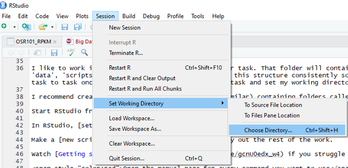
Start RStudio from the Start menu
In RStudio, set your working directory to your scripts folder
Open the filtered data file you created in workshop 1, and make sure it still looks ok by looking at the first few rows as we did in workshop 1
OSR101_final <- read.table("OSR101_final.txt", header=T)
OSR101_final[1:5,1:5]
## A11_Bie A135_Reg A136_Roc A144_She A155_Ste
## A_JCVI_10003 5.593431 2.574767 2.429578 3.794030 7.921821
## A_JCVI_10018 10.619471 7.443781 8.998179 4.292112 8.903025
## A_JCVI_10019 2.076349 2.097265 2.724073 1.931506 2.380547
## A_JCVI_10026 2.022319 2.543542 3.243398 2.785690 2.570395
## A_JCVI_10036 1.334796 1.101064 1.678618 1.738355 1.008232Preparing data for analysis
In this workshop, we want to see if any of the genes may be linked to a trait of interest. Let’s take a look at some trait data for these accessions
gluc <- read.delim("http://www-users.york.ac.uk/~ah1309/BigData/data/Glucosinolates.txt", header=T)
gluc
## Line Trait
## 1 A11_Bie 83.7
## 2 A155_Ste 16.2
## 3 A168_TEM 17.7
## 4 A176_Ver 17.6
## 5 A18_Bro 6.3
## 6 A187_Xia 45.4
## 7 A188_Zho 20.7
## 8 A25_Cap 21.1
## 9 A42_Dar 27.9
## 10 D128_Q10 79.3
## 11 D131_Raf 86.1
## 12 D173_TOP 40.0
## 13 D181_WESD 12.7
## 14 D6_APE 17.1
## 15 D7_APExGIN 58.8
## 16 D75_INCxCON 12.7
## 17 IB02_AbuN 20.8
## 18 IB100_Maj 48.2
## 19 IB106_MoaR 80.0
## 20 IB110_N01D_1330 17.8
## 21 IB111_N02D_1952 15.3
## 22 IB120_Palm 14.9
## 23 IB125_POH285B 14.2
## 24 IB130_Qui 114.3
## 25 IB133_Ram 48.4
## 26 IB141_SenNZ 75.5
## 27 IB143_ShaxWin 29.8
## 28 IB151_SloK 64.7
## 29 IB16_Bra 23.9
## 30 IB164_Tai 82.7
## 31 IB178_Vig 97.1
## 32 IB180_Vis 17.9
## 33 IB184_Yor 82.9
## 34 IB21_Cab 16.2
## 35 IB23_Can 80.5
## 36 IB24_CanxCou 17.9
## 37 IB28_Cas 27.8
## 38 IB29_Cat 17.0
## 39 IB37_ColxNic 19.5
## 40 IB45_Dim 23.8
## 41 IB49_Dup 13.8
## 42 IB50_DwaE 99.8
## 43 IB52_EngG 103.0
## 44 IB53_Erg 92.7
## 45 IB57_Exc 35.1
## 46 IB60_Fla 22.9
## 47 IB70_HanxGas 58.1
## 48 IB73_Hug 10.6
## 49 IB86_LemM 74.3
## 50 IB91_LicxExp 17.6
## 51 IB99_MadxRec 14.2
## 52 NIN 56.1
## 53 TAP 29.5This file has a column of accession names that matches your data (Line), and a column giving percentage of glucosinolates in the seed oil (Trait)
We can merge this with our expression data using the merge function, but first we should set the rownames from the column named Line
rownames(gluc) <- gluc$Line
gluc
## Line Trait
## A11_Bie A11_Bie 83.7
## A155_Ste A155_Ste 16.2
## A168_TEM A168_TEM 17.7
## A176_Ver A176_Ver 17.6
## A18_Bro A18_Bro 6.3
## A187_Xia A187_Xia 45.4
## A188_Zho A188_Zho 20.7
## A25_Cap A25_Cap 21.1
## A42_Dar A42_Dar 27.9
## D128_Q10 D128_Q10 79.3
## D131_Raf D131_Raf 86.1
## D173_TOP D173_TOP 40.0
## D181_WESD D181_WESD 12.7
## D6_APE D6_APE 17.1
## D7_APExGIN D7_APExGIN 58.8
## D75_INCxCON D75_INCxCON 12.7
## IB02_AbuN IB02_AbuN 20.8
## IB100_Maj IB100_Maj 48.2
## IB106_MoaR IB106_MoaR 80.0
## IB110_N01D_1330 IB110_N01D_1330 17.8
## IB111_N02D_1952 IB111_N02D_1952 15.3
## IB120_Palm IB120_Palm 14.9
## IB125_POH285B IB125_POH285B 14.2
## IB130_Qui IB130_Qui 114.3
## IB133_Ram IB133_Ram 48.4
## IB141_SenNZ IB141_SenNZ 75.5
## IB143_ShaxWin IB143_ShaxWin 29.8
## IB151_SloK IB151_SloK 64.7
## IB16_Bra IB16_Bra 23.9
## IB164_Tai IB164_Tai 82.7
## IB178_Vig IB178_Vig 97.1
## IB180_Vis IB180_Vis 17.9
## IB184_Yor IB184_Yor 82.9
## IB21_Cab IB21_Cab 16.2
## IB23_Can IB23_Can 80.5
## IB24_CanxCou IB24_CanxCou 17.9
## IB28_Cas IB28_Cas 27.8
## IB29_Cat IB29_Cat 17.0
## IB37_ColxNic IB37_ColxNic 19.5
## IB45_Dim IB45_Dim 23.8
## IB49_Dup IB49_Dup 13.8
## IB50_DwaE IB50_DwaE 99.8
## IB52_EngG IB52_EngG 103.0
## IB53_Erg IB53_Erg 92.7
## IB57_Exc IB57_Exc 35.1
## IB60_Fla IB60_Fla 22.9
## IB70_HanxGas IB70_HanxGas 58.1
## IB73_Hug IB73_Hug 10.6
## IB86_LemM IB86_LemM 74.3
## IB91_LicxExp IB91_LicxExp 17.6
## IB99_MadxRec IB99_MadxRec 14.2
## NIN NIN 56.1
## TAP TAP 29.5We also need to transpose (swap the dimensions) of our expression data so that the lines are the rows as they are in the trait data.
This is easy in R, we can just create a new object called tOSR and use the t function to transpose the data. Take another look at the file afterwards
tOSR <- t(OSR101_final)
tOSR[1:5,1:5]
## A_JCVI_10003 A_JCVI_10018 A_JCVI_10019 A_JCVI_10026 A_JCVI_10036
## A11_Bie 5.593431 10.619471 2.076349 2.022319 1.334796
## A135_Reg 2.574767 7.443781 2.097265 2.543542 1.101064
## A136_Roc 2.429578 8.998179 2.724073 3.243398 1.678618
## A144_She 3.794030 4.292112 1.931506 2.785690 1.738355
## A155_Ste 7.921821 8.903025 2.380547 2.570395 1.008232Now we are ready merge the two objects by their rownames. Take a look - the trait data should be in the new ORSmerge object along with the expression data.
OSR_merge <- merge(gluc, tOSR, by="row.names")
OSR_merge[1:5,1:5]
## Row.names Line Trait A_JCVI_10003 A_JCVI_10018
## 1 A11_Bie A11_Bie 83.7 5.593431 10.619471
## 2 A155_Ste A155_Ste 16.2 7.921821 8.903025
## 3 A168_TEM A168_TEM 17.7 4.283325 6.187312
## 4 A176_Ver A176_Ver 17.6 5.622508 7.067371
## 5 A18_Bro A18_Bro 6.3 6.735284 4.684116We need to clean this file up a bit by setting the rownames and removing some unnecessary columns. Notice the slight change to remove the first two columns instead of one
rownames(OSR_merge) <- OSR_merge$Line
OSR_merge <- OSR_merge[,-c(1:2)]
OSR_merge[1:5,1:5]
## Trait A_JCVI_10003 A_JCVI_10018 A_JCVI_10019 A_JCVI_10026
## A11_Bie 83.7 5.593431 10.619471 2.076349 2.022319
## A155_Ste 16.2 7.921821 8.903025 2.380547 2.570395
## A168_TEM 17.7 4.283325 6.187312 2.901607 3.458517
## A176_Ver 17.6 5.622508 7.067371 2.862368 2.955425
## A18_Bro 6.3 6.735284 4.684116 4.356354 1.879341Much better! Check the dimensions using the dim function. They may have changed if there was trait data for only some of the lines…
Linear models
Now we have our trait data and gene expression data in one object, let’s do some stats on them. First of all, let’s take a look at the first gene, and plot it against the trait data. This may look complicated, but it just says to plot column 2 against the column called “Trait”, and set the labels for the plot.
plot(OSR_merge[,2], OSR_merge$Trait, ylab="Glucosinolates", xlab=paste("RPKM for gene", colnames(OSR_merge[2])))
It looks like there may be a slightly negative relationship between the trait and gene expression for this gene. Let’s plot the graph again and use a linear model using a function called lm to fit a linear model to the data. We can then use this to fit a line through the data points on the plot
#Linear model using lm function
lm1 <- lm(OSR_merge$Trait~OSR_merge[,2])

#plot column 2 against "Trait" column, and use abline to draw a line based on the linear regression
plot(OSR_merge[,2], OSR_merge$Trait, ylab="Glucosinolates", xlab=paste("RPKM for gene", colnames(OSR_merge[2])))
abline(lm1)
Maybe a slight negative relationship, but is it significant? We can test this using an anova!
anova(lm1)## Analysis of Variance Table
##
## Response: OSR_merge$Trait
## Df Sum Sq Mean Sq F value Pr(>F)
## OSR_merge[, 2] 1 621 621.42 0.6388 0.4278
## Residuals 51 49609 972.73Oh, not significant at all, but that would be too easy anyway!
We can output some other details about this test using some other commands. coefficients will give us the gradient and intercept of the line we drew on the plot, and summary will give us all of the test statistics
#Coefficients
lm1$coefficients
## (Intercept) OSR_merge[, 2]
## 48.889721 -1.340283#Summary
summary(lm1)##
## Call:
## lm(formula = OSR_merge$Trait ~ OSR_merge[, 2])
##
## Residuals:
## Min 1Q Median 3Q Max
## -35.15 -25.09 -16.04 29.07 69.35
##
## Coefficients:
## Estimate Std. Error t value Pr(>|t|)
## (Intercept) 48.890 9.287 5.264 2.84e-06 ***
## OSR_merge[, 2] -1.340 1.677 -0.799 0.428
## ---
## Signif. codes: 0 '***' 0.001 '**' 0.01 '*' 0.05 '.' 0.1 ' ' 1
##
## Residual standard error: 31.19 on 51 degrees of freedom
## Multiple R-squared: 0.01237, Adjusted R-squared: -0.006994
## F-statistic: 0.6388 on 1 and 51 DF, p-value: 0.4278If we want to save any of these results, we need to coerce them into dataframes, and select individual results. Here I’m going to save each important result as a separate object
#Row 1 of the Anova table
anova <- as.data.frame(anova(lm1)[1,])
#Intercept of regression line
intercept = as.data.frame(coefficients(lm1))[1,1]
#Gradient of regression line
gradient = as.data.frame(coefficients(lm1))[2,1]
#R2 (correlation coefficient)
R2 <- as.data.frame(summary(lm1)$r.squared)
Now it would be nice to join all of these in the same object
We can use the c function to stick everything together
result1 <- as.data.frame(c(anova, R2, intercept, gradient))
result1
## Df Sum.Sq Mean.Sq F.value Pr..F. summary.lm1..r.squared
## 1 1 621.4223 621.4223 0.6388424 0.4278372 0.01237135
## X48.8897208547186 X.1.34028278394752
## 1 48.88972 -1.340283Not bad, we’ll fix the horrible column names and add rownames back in later.
“For” loops
So, now we want to do this test and output these results, for all of the genes in the dataset. This will take a while by hand, so we should instruct R to do this for us.
The simplest way to do this is to write a “for” loop. These seem complicated at first, but the structure is quite simple. You just define the data you need to loop through, and surround what you want to do each time in curly brackets.
First, let’s tell the loop where to stop! We can count the total number of columns using the ncol function
numcol <- ncol(OSR_merge)Next, lets create an empty dataframe with 8 columns for our results to go into called results
results <- as.data.frame(matrix(nrow = 0, ncol = 8))Onto the loop! We need to run the whole “for”" loop all at once, so first, let’s look at each individual part.
The first part of the function will tell r which rows to loop though. We want to loop our test through each column of gene expression data which starts in column 2 and ends at numcol.
#for (i in 2:numcol){The next part of the loop will run the linear model, but this time, we will use i (which will loop from 2 to numcol) instead of an individual column number.
#lm1 <- lm(OSR_merge$Trait~OSR_merge[,i])Next, we will output and arrange our results as before
#anova <- as.data.frame(anova(lm1)[1,])
#intercept = as.data.frame(coefficients(lm1))[1,1]
#gradient = as.data.frame(coefficients(lm1))[2,1]
#R2 <- as.data.frame(summary(lm1)$r.squared)
#result1 <- as.data.frame(c(anova, R2, intercept, gradient))
Finally, we will paste our results into our new results dataframe using rbind. This only works if both dataframes have the same column names, so we’ll make sure they do! Finally, close the curly bracket
#colnames(results) <- colnames(result1)
#results <-rbind(results, result)
#}
Ok, here’s the full “for” loop… Don’t forget to run the whole thing in one go!
for (i in 2:numcol){
lm1 <- lm(OSR_merge$Trait~OSR_merge[,i])
anova <- as.data.frame(anova(lm1)[1,])
intercept = as.data.frame(coefficients(lm1))[1,1]
gradient = as.data.frame(coefficients(lm1))[2,1]
R2 <- as.data.frame(summary(lm1)$r.squared)
result1 <- as.data.frame(c(anova, R2, intercept, gradient))
colnames(results) <- colnames(result1)
results <-rbind(results, result1)
}
Lets take a look at the first few rows of our results file!
results [1:5,]## Df Sum.Sq Mean.Sq F.value Pr..F. summary.lm1..r.squared
## 1 1 621.42226 621.42226 0.63884240 0.4278372 0.0123713541
## 2 1 29.86376 29.86376 0.03033915 0.8624125 0.0005945316
## 3 1 470.69649 470.69649 0.48242565 0.4904779 0.0093706860
## 4 1 133.66851 133.66851 0.13607770 0.7137389 0.0026610898
## 5 1 155.57474 155.57474 0.15844805 0.6922509 0.0030972020
## X39.8734375897093 X0.370848391401888
## 1 48.88972 -1.3402828
## 2 40.44312 0.2956792
## 3 51.01240 -2.7162996
## 4 47.96460 -2.4231560
## 5 36.88214 3.8151561We need to put the rownames back on and sort out the column names
rownames(results) <- colnames(OSR_merge[,2:numcol])
colnames(results) <- c("Df", "Sum.Sq", "Mean.Sq", "F.value", "P.value", "R2", "Intercept", "Gradient")
results[1:5,]
## Df Sum.Sq Mean.Sq F.value P.value R2
## A_JCVI_10003 1 621.42226 621.42226 0.63884240 0.4278372 0.0123713541
## A_JCVI_10018 1 29.86376 29.86376 0.03033915 0.8624125 0.0005945316
## A_JCVI_10019 1 470.69649 470.69649 0.48242565 0.4904779 0.0093706860
## A_JCVI_10026 1 133.66851 133.66851 0.13607770 0.7137389 0.0026610898
## A_JCVI_10036 1 155.57474 155.57474 0.15844805 0.6922509 0.0030972020
## Intercept Gradient
## A_JCVI_10003 48.88972 -1.3402828
## A_JCVI_10018 40.44312 0.2956792
## A_JCVI_10019 51.01240 -2.7162996
## A_JCVI_10026 47.96460 -2.4231560
## A_JCVI_10036 36.88214 3.8151561Much better. Save it for next time!
write.table(results, "Results.txt", quote=F, sep="\t")For next time
Try completing these tasks using your results from the full dataset. The full dataset is here if you need it.
save.image("Workshop2.Rda")