Introduction to module and RStudio
Emma Rand

Introduction
Session overview
This session has been designed assuming you have carried out the prior Independent Study as recommended. If you have not carried that out and have some familiarity with coding (not necessarily in R), you may be able to dive in but otherwise I suggest using this workshop time to carry out the independent study first.
In this introduction you will start working with RStudio. The independent study equips you to use the help manual, install R and Rstudio on your own computer and uses DataCamp again to cover some more fundmental R.
Learning Outcomes
By actively following the lecture and practical and carrying out the independent study before and after the contact hours the successful student will be able to:
- to explain why we need statistical tests and the logic of hypothesis testing (MLO 1)
- use the R command line as a calculator and to assign variables (MLO 3)
- create and use the basic data types in R (MLO 3)
- find their way around the RStudio windows (MLO 3)
- create, use and save a script file to run r commands (MLO 3)
- search and understand manual pages (MLO 3)
Philosophy
Workshops are not a test. It is expected that you often don’t know how to start, make a lot of mistakes and need help. Do not be put off and don’t let what you can not do interfere with what you can do. You will benefit from collaborating with others and/or discussing your results.
The lectures and the workshops are closely integrated and it is expected that you are familar with the lecture content before the workshop. You need not understand every detail as the workshop should build and consolidate your understanding. You may wish to refer to the slides as you work through the workshop schedule.
Slides
Introduction to module and RStudio: pdf (recommended) / pptx
Your responses from TurningPoint.

Artwork by @allison_horst
What are R and RStudio?
R is a free, open source language for statistical computing and graphics.
Because R is an Open Source project there is an amazing community of R users (for examples: R Bloggers, stackoverflow and Cross Validated ) that is informative and helpful for users at all levels.
RStudio is an “Integrated Development Environment” or IDE for R. Using R in an RStudio makes it easier to do many things. The DataCamp tutorials are modelled on RStudio.
Getting started with RStudio
You may be able get started in RStudio just by following the instructions below with some intuition but if not, try watching Getting started with RStudio.
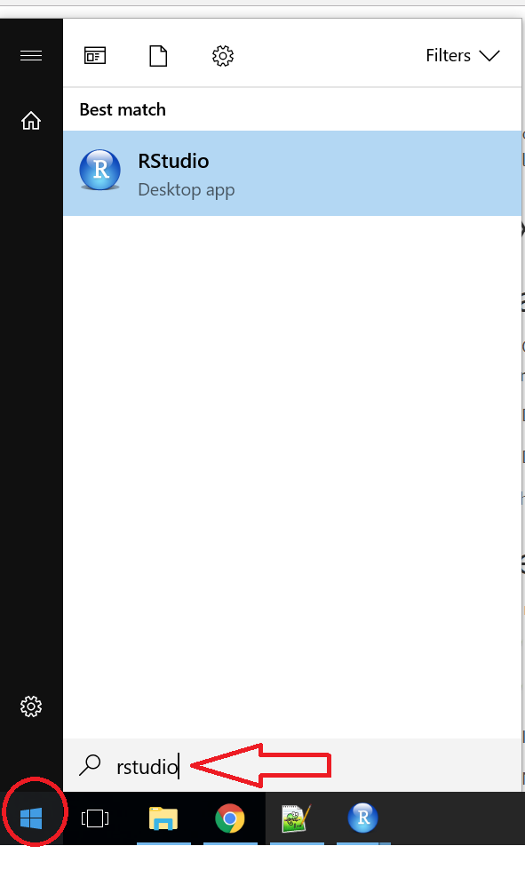
 Start RStudio from the Start menu. My RStudio Anatomy may be a useful reference

In Windows explorer, make yourself a folder for 17C Data Analysis work.
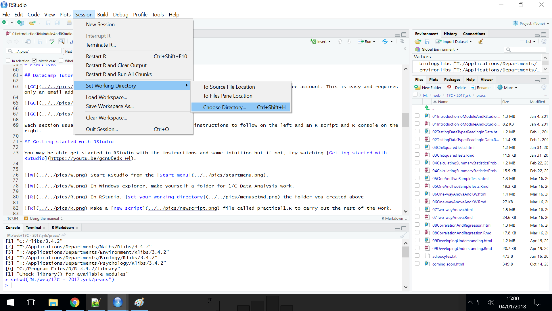
 In RStudio, set your working directory the folder you created above
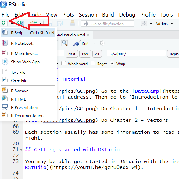
Make a new script then save it with a name like practical1.R to carry out the rest of the work.
Try using some of the commands you used in the DataCamp tutorial.
Your first graph
In this first exercise, you will create vectors of some data, plot them using the ‘base’ plotting system, and learn how to use the manual to customise the plot.
We will work some data on the number of males in 64 bird nests with a clutch size of 5. The data are as follows:
| No. males | No.nests |
|---|---|
| 0 | 4 |
| 1 | 13 |
| 2 | 14 |
| 3 | 15 |
| 4 | 13 |
| 5 | 5 |
| Total | 64 |
Make a vector n that holds the numbers 0 to 5. Write your command in the script file and run it using the Run button or doing Control-R. In either case you need to have your cursor on the line you want to execute.
Examine the ‘structure’ of the n object using str()
Create a vector called freq containing the numbers of nests with 0 to 5 males.
check sum(freq) gives the answer you expect
Now for your first figure.
Create simple barplot with barplot(freq)

Using the manual
The barplot doesn’t have any numbers to say what each bar represents or any axis labels. We need to add arguments to the barplot() command. Functions do something and their arguments specify what object to do the function to and how exactly to do it. Many arguments have defaults so you need only supply an object.
Open the manual page using ?barplot and look over the Arguments
Add names using the names.arg argument:

Now use the manual to try to make the following changes to the graph:
Add labels for both axes so it looks like this:

Make all the bars red so it looks like this:

Make the bars alternating red, blue, and yellow so it looks like this:

Important: the data you have just been working with was in the form of a frequency table. Much more often you will have the ‘raw’ data which you need to summarise.
Your second graph
In this second exercise, you will generate some random data and plot them using the ggplot plotting system. At first, ggplot can seem to need more coding than the ‘base’ plotting system but it makes even slightly more complex graphs easier to do and very complex graphs no more difficult. We will use ggplot a lot.
ggplot wants the data it plots to be inside a ‘dataframe’.
We are going to generate data which are the number of males in 64 nests. We do this with a function called rbinom() which generates random numbers from a binomial distribution. You do not need to understand what a binomial distribution is or why it is appropriate here. All you need to appreciate is that it is a way to make 64 numbers which represent the number of males in a nest.
We can use the rbinom() function can put the data into a ‘dataframe’ like this:
nest_data <- data.frame(n_males = rbinom(n_of_nests, clutch_size, p_of_male))
nest_data is just a name we have given the dataframe and n_males is a column in that data frame. We could put numbers inside the rbinom() function:
nestdata <- data.frame(n_males = rbinom(64, 5, 0.5)) but good programming practice is to create variables to hold those values, and put the variables in the function.
Make the three variables for the number of nests, the clutch size and the the probability an individual is male:
Now generate the data:
Examine the ‘structure’ of the nest_data object using str()
If you click on nest_data in the Environment pane, a spreadsheet-like view of it will appear.

To use ggplot we first tell R using a library statement. ggplot2 is the name of the collection (called a package) of ggplot functions.
Now plot the data like this:

Notice that ggplot has automatically counted the number of zeros, ones, twos, etc and plotted those.
You can add an axis label like this:

Notice that the ggplot syntax is a bit different to the ‘base’ plotting syntax.
Can you work out how to customise the plot at all?
Well Done!

Artwork by @allison_horst
Independent study
Please note that the next workshop session assumes you have carried out the independent study.
1. Getting help in RStudio
Being able to use the manual is a threshold concept in R. You get a feel for the structure and pattern of commands much quick if you make a habit of briefly reading the manual for the commands you are using.
 Watch Getting help in RStudio
2. More DataCamp
Do Chapter 4 - Factors
Do Chapter 5 - Dataframes
Note, you do not need to do chapters 3 and 6 unless you want to.
3. Reading
From Dani Navarro’s Learning statistics with R: Read 1.1 On the psychology of statistics section of the chapter 1 Why do we learn stastistics? Approx 5 minutes.
From Sharon Machlis’ Practical R for Mass Communication and Journalism: Read Why programming? and Wny R?. Approx 5 minutes.
Getting R on your own computer
R is free and easy to install. Putting it on your own computer will make easier for you to practice R when it suits you. You will need to:
- First download and install R from http://www.r-project.org/
- Then download and install RStudio from https://www.rstudio.com/
There is a video of the steps Installing R and RStudio on your own pc
The Code files
These contain answers and code even though they do not appear on the webpage itself.
Rmd file The Rmd file is the file I use to compile the practical. Rmd stands for R markdown allow R code and ordinary text to be inter weaved to produce well-formatted reports including webpages.
Plain script file This is plain script (.R) version of the practical
