 d
d
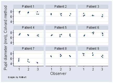
Figure 1 shows the first 9 patients from a study of 28, where each patient was measured 3 times by each of 3 observers.
Figure 1. Pupil diameters measured 3 times by each of 3 observers,
first 9 patients from a study of 28.
 d
d
Inspection of the data suggests that there is more variation between observations by different observers than when the same observer measures a patient. Patient 6 is a good example. The variability between measurements on the same subject by different observers is called observer variation.
We can estimate the effects of observer variation using the same kinds of statistics as we do for measurement error by the same observer: within-subject standard deviation and coefficient of variation, and correlation coefficients, usually ICCs. We can estimate these statistics for different observers on the same occasion, on different occasions, and so on.
For the data of Figure 1 (all 28 subjects) the intra-observer within-subject standard deviation was sw = 0.38 mm. The corresponding ICC = 0.80. The inter-observer within-subject standard deviation was 0.48 and the ICC was 0.72. The standard deviation is greater with different observers and the ICC is smaller, both reflecting the greater error when different observers used this measurement.
Many designs can be used to investigate observer variation, depending on the purpose of the investigation and the resources available. There are several reasons for carrying out observer comparison studies.
Sometimes our focus of interest is the properties of the measurement method itself:
Sometimes the focus may be on the observers rather than the measurement method:
This variety of purpose leads to a variety of designs and analyses. For some purposes, such as demonstrating the possibility of the measurement being applied by different observers or observer training, the number of observers is fixed by the objective. For others, the main problem is getting enough observers to have a reasonable sample to represent observers in general.
The usual design is to get several observers each to measure several subjects, preferably more than once. All we need to do is to ask a sample of observers, representative of the observers whose variation we wish to study, to make repeated observations on each of a sample of subjects, the order in which observers make their measurements being randomized. We then ask by how much the variation between measurements on the subject is increased when these measurements are made by different observers.
In practice, the ideal design of a representative sample of observers making repeated measurements on each of a sample of subjects is almost always impossible in the study of clinical measurements. There are several reasons for this:
For these reasons, most observer comparison studies are a compromise between the ideal study design and practical and ethical limitations.
There is one other possible design which might be considered ideal. This is to have every subject measured by two different observers, using new observers every time. We could then use the methods for simple measurement error to estimate the standard deviation within subjects when each measurement is by a different observer. This design is most unlikely to be used in practice, but we may sometimes choose to analyse our data as if it was, ignoring the fact that the same observer is used several times.
One solution to the problem of needing many observers to measure the same subject is to carry out several small replicates of the ideal design and then combine them. An example is the study of the measurement of abdominal circumference by fetal ultrasound shown in Table 1.
| Observer | Subject 1 | Subject 2 | Subject 3 | ||||||
|---|---|---|---|---|---|---|---|---|---|
| 1 | 13.6 | 13.3 | 12.9 | 14.7 | 14.8 | 14.7 | 17.1 | 17.1 | 18.3 |
| 2 | 13.8 | 14.2 | 13.2 | 14.9 | 14.1 | 14.5 | 17.2 | 17.5 | 17.6 |
| 3 | 13.2 | 13.1 | 13.1 | 14.5 | 14.2 | 13.8 | 16.3 | 15.2 | 16.1 |
| 4 | 13.7 | 13.7 | 13.4 | 14.4 | 14.3 | 13.6 | 16.8 | 16.8 | 17.5 |
| Subject 4 | Subject 5 | Subject 6 | |||||||
| 5 | 14.8 | 14.6 | 14.8 | 18.3 | 18.5 | 18.5 | 12.6 | 12.6 | 12.4 |
| 6 | 14.9 | 14.4 | 14.2 | 17.4 | 17.9 | 17.0 | 12.3 | 12.1 | 12.1 |
| 7 | 14.3 | 14.4 | 14.3 | 17.7 | 17.0 | 18.3 | 12.5 | 12.2 | 12.6 |
| 8 | 13.8 | 14.1 | 14.1 | 17.4 | 17.9 | 16.4 | 13.0 | 12.6 | 12.7 |
| Subject 7 | Subject 8 | Subject 9 | |||||||
| 9 | 12.4 | 11.7 | 11.6 | 16.0 | 16.0 | 16.2 | 11.3 | 11.6 | 10.7 |
| 10 | 11.5 | 12.5 | 12.8 | 16.1 | 15.8 | 15.4 | 9.7 | 10.2 | 9.8 |
| 11 | 14.6 | 12.7 | 11.5 | 16.7 | 16.5 | 16.2 | 10.7 | 10.3 | 9.8 |
| 12 | 13.5 | 13.4 | 12.5 | 17.0 | 16.6 | 17.2 | 10.9 | 11.2 | 11.3 |
| Subject 10 | Subject 11 | Subject 12 | |||||||
| 13 | 14.3 | 14.4 | 14.8 | 15.6 | 15.9 | 16.1 | 20.2 | 20.9 | 21.1 |
| 14 | 14.3 | 15.5 | 14.6 | 15.7 | 15.0 | 16.5 | 20.1 | 20.7 | 20.9 |
| 15 | 14.6 | 14.8 | 15.4 | 16.3 | 16.1 | 15.6 | 19.2 | 20.0 | 20.0 |
| 16 | 14.1 | 14.6 | 13.7 | 14.4 | 15.1 | 15.2 | 20.5 | 20.5 | 21.1 |
It was thought feasible for four observers each to make three measurements on a patient. The investigators were able to arrange for three patients to be available for a group of four observers. Thus we have a block of data consisting of four observers, three subjects, and three measurements by each observer on each subject. This is the ideal study design, apart from the small numbers of observers and subjects involved. Now we can repeat this, using four more observers and three more patients, and combine the two studies. Thus we increase the numbers of observers and subjects without putting too many demands on either. In the study shown in Table 1, there were four replications, so that altogether sixteen observers each made three measurements on three patients, and there were twelve patients in all.
This design enables unlimited numbers of observers and patients to be studied without undue stress on either subjects or observers. It also lends itself very neatly to a multicentre study, where small groups of observers could make their measurements in different institutions.
Another strategy which has been used is to construct a physical model of the object to be measured. Obvious advantages are that the model can then be measured as often as required and the true value is known. For example, Moertel and Hanley (1976) made model tumours from 12 solid spheres, arranged in random order on a soft mattress and covered with foam rubber 0.5 inches thick for the six smaller spheres and 1.5 inches thick for the six larger spheres. They then invited 16 experienced oncologists to measure the diameter of each sphere, each observer using the technique and equipment which they routinely used in clinical practice.
There are other ways in which observer variation can be studied without the presence of the subject. When physical contact is not necessary, a video recording of a patient can be used as a subject and measured repeatedly. For example, Falkowski et al. (1980) used video recordings of psychiatric interviews to investigate observer variation in assessment of ego state. It may be possible to present the same subject more than once, as in the British Hypertension Society training film of blood pressure measurements. In this, the manometer is shown while the Korotkov sound is heard on the sound track. Each recording is included twice, but the observers are not told and do not notice this and so there is no bias in the second reading from knowledge of the first.
Such artificial measurement situations are very useful for investigating some of the sources of variation in a measurement and for observer training, but we cannot be sure that they embody all the sources of variation present in practice. They cannot entirely replace investigations of measurement variation in the living subject.
In this lecture we shall consider only continuous outcomes, i.e. measurements, as opposed to categorical ones. We deal with the latter separately using Cohens kappa statistics.
The full data for the pupil diameter study are shown in Table 2. To estimate the increase in variation when different observers are used, we use analysis of variance. Compared to the simple measurement error problem, the analysis of variance is more complicated, because we have more sources of variation. The variation for repeated observations by the same observer on the same subject we will call sw2, as before. The variation between subjects, that is between the true values of the quantity being measured, will be sb2, as before. By true value we mean the average value we would get from many measurements by many different observers.
The variation due to observers is made up of two different components. An observer may have a bias, a fixed effect where that observer consistently measures higher or lower than others. There may also be a random effect, which we will call the heterogeneity, where the observer measures higher than others for some subjects and lower for others.
The meaning of heterogeneity may be obscure, and a thought experiment may make it clearer. In the film 10 (Edwards 1979), Dudley Moore scores feminine attractiveness out of ten. Suppose we wish to estimate the observer variation of this highly subjective measurement. We persuade several observers to rate several subjects, and repeat the rating the several times. Now there will be an overall mean rating, for all subjects by all observers on all occasions. Some subjects will receive higher mean scores than others and this variation about the overall mean is measured by sb2. If we get the same observer to rate the same subject several times, the ratings will vary. The variation between the individual measurement and the mean for that observer's measurement of that subject is measured by the measurement error, sw2. Some observers will be more generous in their ratings than others. The variation of the observer means about the overall mean is measured by another variance, so2. For a given observer, this is the bias, the tendency to rate high or low. What about the heterogeneity? It is well known that people tend to be attracted to partners who look like them. Tall, thin women marry tall, thin men, and short, fat men marry short, fat women, for example. (Take a good look at your friends if you don't believe this.) Thus Bland, who is short, may give higher ratings to short women than to tall ones, and Altman, who is tall, may give higher ratings to tall women than to short, even though their overall mean ratings may be the same. This is the heterogeneity, or observer times subject interaction, and it may be just as important as the observer bias. It comes from the difference between the mean rating for a given subject by a given observer and the rating we would expect for this subject and observer given the mean rating over all observers for the subject and the mean rating over all subjects by the observer.
Physical measurements can behave in the same way. Measured blood pressure is said to be higher when subject and observer are of opposite sex than when they are the same sex. If both observers and subjects include both sexes, this will contribute to heterogeneity. In general, there may be unknown observer and subject factors which contribute to heterogeneity and our method of analysis must allow for the possibility of their presence. We will denote the extra variability in measurements due to this heterogeneity by sh2.
The final measurement is made up of the overall mean, the difference from the mean for that particular subject, the difference from the mean for the observer, the heterogeneity, and the measurement error. We assume that the effects of subject, observer and measurement error are added.
Hence we have four different variances, and if we have measurements on different subjects made by different observers, the variance will be the sum of all of them:
s2 = sb2 + so2 + sh2 + sw2
To recap:
These four variances are called the components of variance.
We shall assume that all the errors, between observers, the heterogeneity, and the measurement error, are independent of one another and of the magnitude of the measurement. This means, for example, that the measurement error for one observer is the same as the measurement error for another. If we do not assume this, we cannot estimate the errors. We shall also assume that they follow a Normal distribution, so that we can estimate confidence intervals for our estimates.
The assumptions that these variables are Normal, independent and have uniform variances are quite strong, particularly that the measurement error variance sw2 is the same for all observers, but it is very difficult to proceed without them.
We can estimate the components of variance by analysis of variance, which is straightforward provided we have the same number of repeated measurements by each observer on each subject.
For the pupil diameter data, the anova table is:
| Source | Sum of squares | Degrees of freedom | Mean square | F ratio | P value |
|---|---|---|---|---|---|
| Subject | 153.74107 | 27 | 5.69411376 | 39.31 | 0.0000 |
| Observer | 3.43056 | 2 | 1.71527778 | 11.84 | 0.0000 |
| Subject × Observer | 19.62500 | 54 | 0.36342593 | 2.51 | 0.0000 |
| Residual | 24.33333 | 168 | 0.14484127 | ||
| Total | 201.12996 | 251 | 0.80131458 |
We have a row for each source of variation: between subjects, between observers, the subject times observer interaction, and the residual within subject and observer.
We can estimate the four variances from the following table, which shows the expected values of mean squares in a two-way analysis of variance table for o observers each measuring n subjects m times:
| Source of variation | Degrees of freedom | Mean square |
|---|---|---|
| Total | mno – 1 | |
| Subjects | n – 1 | mosb2 + msh2 + sw2 |
| Observers | o – 1 | mnso2 + msh2 + sw2 |
| Subjects × observers | (n – 1)(o – 1) | msh2 +sw2 |
| Residual error | (m – 1)no | sw2 |
There is no need to remember all these multipliers, but we can note that each variance is multiplied by the number of observations made at one level of the factor. For example, each subject is measured by o observers m times, and its multiplier is mo. For the pupil diameter data, m = 3, o = 3, n = 28.
The components of variance are found as follows:
sw2 = 0.14484127, sw = 0.38
sh2 = (0.36342593 – 0.14484127)/3 = 0.07286155, sh = 0.27
so2 = (1.71527778 – 0.36342593)/(3 × 28) = 0.01609347, so = 0.17
sb2 = (5.69411376 – 0.36342593)/(3 × 3) = 0.59229865, sb = 0.77
The intra-observer within-subject standard deviation is therefore 0.38, and the intraclass correlation coefficient is
ICC = sb2/(sb2 + sw2) = 0.59229865/(0.59229865 + 0.14484127) = 0.80.
The inter-observer within-subject standard deviation is therefore
square root (so2 + sh2 + sw2) =
square root (0.01609347 + 0.07286155 + 0.14484127) = 0.48
and the ICC is
sb2/( sb2 + so2 + sh2 + sw2) = 0.59229865/(0.59229865 + 0.01609347 + 0.07286155 + 0.14484127) = 0.72.
Note that both main observer effect and the eye times observer interaction (heterogeneity) are highly significant (P<0.0001).
For the estimation of observer variation, the same assumptions are made about the data as for measurement error. We assume that the within-subjects standard deviation is independent of the mean, that the distribution within the subject is approximately Normal, and for correlation we require a representative sample and Normal distribution for the measurement itself, not just the errors.
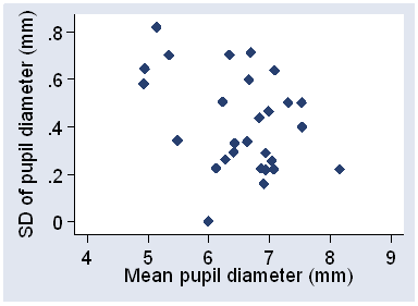
We can check these assumptions graphically. For the pupil diameter data, Figure 2 shows the within-subject standard deviation against subject mean.
Figure 2. Standard deviation against subject mean for the pupil diameter data.
 d
d
It appears that standard deviation decreases as the magnitude increases, an unusual property. Pupil diameter is measured after the eye has become accustomed to darkness and so the pupil is relaxed and at its fullest extent. It is therefore near to its upper limit, which may explain this.
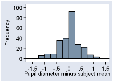
We can check the distribution of the errors within the subject by calculating the difference from the subject mean for each observation and drawing a histogram (Figure 3).
Figure 3. Histogram of differences from subject mean for the pupil diameter data.
 d
d
This looks fairly symmetrical, though the peak is a bit too high for a Normal distribution. The plus or minus 2 SD limits should work fairly well.
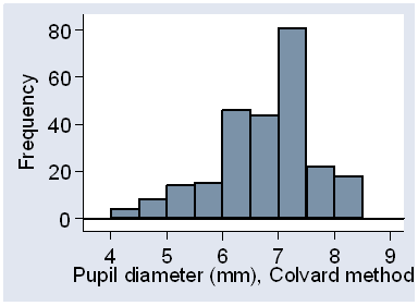
There is a negative skewness in the distribution, as is shown by the histogram of all observations (Figure 4).
Figure 4. Histogram of all observations, for the pupil diameter data.
 d
d
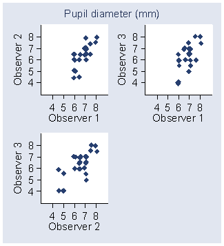
We would not usually mix repeated observations from different subjects in this way, but in this case all we want is a visual impression and it will not cause any problems. This deviation from the Normal is also shown by the scatter plots for observers (Figure 5).
Figure 5. Scatter plots for observers, first measurement,
for the pupil diameter data.
 d
d
These show several things: that Observer 1 did not record low readings and that the observers get closer together for higher pupil diameters, for example. Hence the necessary assumptions are not met for these data and the estimates obtained can only be approximate.
Bland JM. (2005) How do I analyse observer variation studies? (Adobe PDF file)
Falkowski W, Ben-Tovim DI, Bland JM. (1980) The assessment of the ego states. British Journal of Psychiatry, 137, 572-573.
Moertel, C.G. and Hanley, J.A. (1976) The effect of measuring error on the results of therapeutic trials in advanced cancer. Cancer, 38, 388394.
To Measurement in Health and Disease index.
To Martin Bland's M.Sc. index.
This page maintained by Martin Bland.
Last updated: 21 April, 2008.