• Markov Chains
• Notations
• Classification of states
  • Recurrence time
  • Invariant distribution or stationary or equilibrium, or steady-state distribution
    • An example with more than one solutions
  • Limiting distribution
    • Interpretation 1: the proportion of time it spends in state $j$ after running for a long time
      • Expected value of the number of visits
      • An example
    • Interpretation 2: the probability that the process will be in state $j$ after running for a long time
    • An example
    • Another example (a stationary distribution is not necessary a limiting distribution)
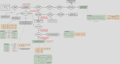
• Summarise in a diagram

Markov Chains

A definition from Probability - An Introduction by Geoffrey Grimmett and Dominic Welsh.

Defintion 12.1 A sequence $X$ of random variables is called a Markov chain if it satisfies the Markov property $$\begin{align*} & \forall n \leq 0 \land i_0, i_1, ..., i_{n+1} \in S \bullet \\ & \qquad \mathbb{P}\left(X_{n+1}=i_{n+1} | X_0 = i_0, X_1 = i_1, ..., X_n=i_n\right) \\ & \qquad = \mathbb{P}\left(X_{n+1}=i_{n+1} | X_n=i_n\right) \end{align*}$$ where $S$ is a countable set called the state space.

Provided $V$ is an initial distribution vector, satisfying $\forall i \in S \bullet V(i) \geq 0 \land \Sigma_{i \in S} V(i) = 1$, and $P$ is a stochastic transition matrix, a random sequence $\bar{X} = \langle X(n) | n \geq 0 \rangle$ is a Markov chain with $V$ and $P$ if $\forall n \geq 0 \land i_0, \dots i_n \in S$, then $$\begin{align*} & \mathbb{P}\left(X_0=i_0,...,X_n=i_n\right) \\ = & V(i_0) * P(i_0, i_1) * P(i_1, i_2) * \dots * P(i_{n-1}, i_n) \end{align*}$$

Notations

• $P_{ij}$ is called one-step transition probabilities (note: directly connected in state transition diagrams)
• $P_{ij}^{(n)}$: called n-step transition probabilities,
  • $\triangleq \mathbb{P}\left(X_n = j | X_0 = i\right)$
  • starting from state $i$, after exact $n$ steps, the probability of being at state $j$
• $P^{(n)}$, called $n$-step transition matrix,
  • the $i$th row and $j$th column of $P^{(n)}$ is just $P_{ij}^{(n)}$
• $i$ lead to $j$, $i \to j$,
  • $\triangleq \left(\exists n \geq 0 \bullet P_{ij}^{(n)} > 0\right)$
  • there is a path from $i$ to $j$ in $n$ steps,
  • if $n=0$, then $i \to i$,
• $i$ and $j$ communicate: $i \leftrightarrow j$
  • $i \to j$ and $j \to i$
  • $i$ and $j$ lead to each other
  • $\leftrightarrow$ is an equivalence relation: reflexive, symmetric, and transitive.
• $C(i) = {j \in S : i \leftrightarrow j}$
  • or $[i]$: the equivalence class of an element $i$ in $S$,
    • Example: S={a, b, c}, ${\displaystyle R=\{(a,a),(b,b),(c,c),(b,c),(c,b)\}}$, here $R$ is an equivalence relation. $[a] = \{a\}$ and $[b]=[c]=\{b, c\}$. The set of all equivalence classes is ${\displaystyle \{\{a\},\{b,c\}\}}$(See here)
  • Equivalence classes or communicating classes,
• $\bar{X}$ (or $S$) is irreducible:
  • a single communicating class, that is, $\forall i, j \in S \bullet i \leftrightarrow j$,
• A subset $C \subseteq S$ is closed,
  • if $\forall i \in C; j \in S \bullet i \to j \implies j \in C$,
  • also $\forall i \in C; j \notin C \bullet P_{ij} = 0$
  • there is no such path leaving from $C$,
  • or called Bottom strongly connected component (BSCC)
    • Strongly connected components (SCCs) are the maximal strongly connected set of states, forming a partition of states.
• State $i$ is called recurrent or persistent,
  • if and only if $\mathbb{P}(T(i) < \infty | X_0 = i) = 1$, where
    • the first passage time: $T(j) = min \{n \geq 1: X_n = j\}$ - the number of steps when the random variable in a chain is at state $j$ again for the first time,
    • the first passage probability: $f_{ij}^{(n)} = \mathbb{P}(T(j) = n | X_0 = i)$,
  • this means if a chain starts at state $i$, it will surely return at state $i$ in finite steps (the first passage time is less than $\infty$),
  • a theorem in terms of $P$: a state $i$ is recurrent if and only if $$\sum_{n=0}^{\infty} P_{ii}^{(n)} = \infty$$
    • the chain will return to state $i$ infinitely often (return again and again, forever)
• State $i$ is transient if it is not recurrent,

Classification of states

Considering a chain starting at state $i$,

• $V(i) = |\{n \geq 1: X_n = i\}|$
  • the number of subsequent visits by the chain to state $i$ again,
• $V(i)$ has a geometric distribution
  • $\mathbb{P}(V(i) = r | X_0 = i) = (1 - f) * f ^ r$ where
    • $r \in \mathbb{N}$
    • $f = f_{ii} = \sum_{n=1}^{\infty} \mathbb{P}(X_n = i | X_0 = i)$ - the return probability,
  • for example, $P = \{0.5, 0.5; 0.3, 0.7\}$, then
    • $V(S_0) = $
• if $\mathbb{P}(V(i) = \infty | X_0 = i) = 1$, then $i$ is recurrent,
• if $\mathbb{P}(V(i) < \infty | X_0 = i) = 1$, then $i$ is transient,
• $\mathbb{E}(i, Z) = \mathbb{E}(Z | X_0 = i)$

Recurrence time

• the first-passage time to $i$:

  • $T(i) = inf \{n \geq 1: X_n = i\}$
  • use $inf$ or $min$ above

• the recurrence time $T(i)$ of $i$, if $X_0 = i$.

• the mean recurrence time of $i$, $\mu(i) = \mathbb{E}(T(i) | X_0 = i)$

  • $=\infty$ if $i$ is transient,
  • $=\sum_{n=1}^{\infty} n*f_{ii}^{(n)}$ if $i$ is recurrent,
    • the summation of products of the time of a recurrence and its corresponding probability

• if $i$ is recurrent,

  • $i$ is null if $\mu(i) = \infty$,
  • $i$ is positive or non-null if $\mu(i) < \infty$.

• the period $d(i)$

  • $d(i) = gcd \{n : P(n, i, i) > 0\}$
    • the greatest common divisor of the set …
  • $i$ is aperiodic if $d(i)=1$,
  • $i$ is periodic if $d(i) > 1$,
  • all states in a communicating class are either aperiodic or periodic with the same period,
  • all communicating classes can be aperiodic or periodic,

• the state $i$ is ergodic if $i$ is aperiodic and positive recurrent.

• if $i \leftrightarrow j$, then both $i$ and $j$

  • have the same period,
  • are recurrent if one is,
  • are positive recurrent if one is,
  • are ergodic if one is.

• a communicating class $C$ can also be regarded as recurrent, transient, ergodic, …

Invariant distribution or stationary or equilibrium, or steady-state distribution

A vector $\pi = [\pi(s_0), \dots \pi(s_n)]$ is called an invariant distribution under the passage of time if

• $\forall i \in S \bullet \pi(i) \geq 0$ and
• $\sum_{i\in S} \pi(i) = 1$,
• $\pi = \pi P$.

Below is from Emma J. McCoy’s lecture note:

• If a finite Markov chain has two or more closed communicating classes, the stationary distributions are not unique,
• If a finite Markov chain has zero or one closed communicating class, then the stationary distribution is unique.

An example with more than one solutions

From here $$P = \begin{bmatrix} 1 & 0 & 0\\ \frac{1}{3} & \frac{1}{3} & \frac{1}{3}\\ 0 & 0 & 1 \end{bmatrix}$$ $$\pi_1 = \begin{pmatrix} \frac{3}{4} & 0 & \frac{1}{4} \end{pmatrix}$$ $$\pi_2 = \begin{pmatrix} \frac{1}{3} & 0 & \frac{2}{3} \end{pmatrix}$$

Both $\pi_1$ and $\pi_2$ satisfy $\pi_1 P = \pi_1$ and $\pi_2 P = \pi_2$

$$P^2 = \begin{bmatrix} 1 & 0 & 0\\ \frac{4}{9} & \frac{1}{9} & \frac{1}{9}\\ 0 & 0 & 1 \end{bmatrix} P^3 = \begin{bmatrix} 1 & 0 & 0\\ \frac{13}{27} & \frac{1}{27} & \frac{13}{27}\\ 0 & 0 & 1 \end{bmatrix} \dots P^{12} = \begin{bmatrix} 1 & 0 & 0\\ \frac{1}{2} & 0 & \frac{1}{2}\\ 0 & 0 & 1 \end{bmatrix} $$

When $n \to \infty$, $$P^n = \begin{bmatrix} 1 & 0 & 0\\ \frac{1}{2} & 0 & \frac{1}{2}\\ 0 & 0 & 1 \end{bmatrix}$$ , there is no limiting distribution.

Limiting distribution

Interpretation 1: the proportion of time it spends in state $j$ after running for a long time

$$\forall j \in S \bullet \pi_j = \lim_{n \to \infty} \frac{1}{n}\sum_{m=1}^{n} p_{ij}^{(m)}$$ here $\pi_j$ may depend on the initial distribution $i$.

Recall that $p_{ij}^{(m)}$ is the probability of a Markov chain at state $j$ after exact $m$ steps when it starts from state $i$, then $\sum_{m=1}^{n} p_{ij}^{(m)}$ is the probability of a chain at state $j$ in $n$ steps when it starts from state $i$. It can also be interpreted as the expected value of the number of visits to $j$ in first $n$ steps (see Expected value of the number of visits). And so $\frac{1}{n}\sum_{m=1}^{n} p_{ij}^{(m)}$ is the proportion of time the chain spends at state $j$ in $n$ steps.

Definition of the limiting distribution

If for all state $j$, $\pi_j$, calculated as above, exists and is independent of the initial state $i$, and $\sum_{j\in S} \pi_j = 1$, then the probability distribution $\pi$ is a limiting distribution.

Expected value of the number of visits

Let $V_j^n$ be the number of visits the chain to state $j$ after exact $n$ steps. \begin{align*} V_j^n & = \begin{cases} 1 & \text{if } X_n = j,\\ 0 & \text{if } X_n \neq j. \end{cases} \end{align*}

Then $\sum_{n=1}^{N} V_j^n$ means the number of visits to state $j$ in $N$ steps. \begin{align*} & \mathbb{E}\left(\left(\sum_{n=1}^{N} V_j^n\right) | X_0 = i\right) \\ & = \sum_{n=1}^{N} \mathbb{E}\left(V_j^n | X_0 = i\right) \\ & = \sum_{n=1}^{N} \left(1 \times \mathbb{P}\left(V_j^n=1 | X_0 = i\right) + 0 \times \mathbb{P}\left(V_j^n=0 | X_0 = i\right)\right) \\ & = \sum_{n=1}^{N} \mathbb{P}\left(V_j^n=1 | X_0 = i\right) \\ & = \mbox{(Definition of $V_j^n$)}\\ & \qquad \sum_{n=1}^{N} \mathbb{P}\left(X_n = j | X_0 = i\right)\\ & = \sum_{n=1}^{N} p_{ij}^{(n)} \end{align*}

An example

$$P = \begin{bmatrix} \frac{1}{4} & \frac{1}{2} & \frac{1}{4}\\ \frac{1}{3} & 0 & \frac{2}{3}\\ \frac{1}{2} & 0 & \frac{1}{2} \end{bmatrix}$$ $$\forall n \geq 11 \bullet P^n = \begin{bmatrix} \frac{3}{8} & \frac{3}{16} & \frac{7}{16}\\ \frac{3}{8} & \frac{3}{16} & \frac{7}{16}\\ \frac{3}{8} & \frac{3}{16} & \frac{7}{16} \end{bmatrix}$$ $$\lim_{n \to \infty} \frac{1}{n}\sum_{m=1}^{n} P^{(m)}=\begin{bmatrix} \frac{3}{8} & \frac{3}{16} & \frac{7}{16}\\ \frac{3}{8} & \frac{3}{16} & \frac{7}{16}\\ \frac{3}{8} & \frac{3}{16} & \frac{7}{16} \end{bmatrix}$$ In this case, $P^{(n)}$ converges to a matrix whose each row is the same. Actually, each row corresponds to $p_i^{(n)}$ which is related to the initial distribution. So eventually, the $p_{ij}^{(n)}$ is independent of $i$ because each row is the same.

Interpretation 2: the probability that the process will be in state $j$ after running for a long time

A distribution $\pi = [\pi_0, \pi_1, …, \pi_n]$ is called a limiting distribution of $X_n$ if $$\forall i, j \in S \bullet \pi_j = \lim_{n \to \infty} \mathbb{P}(X_n = j | X_0 = i)$$

Also we can write it as $$\forall i, j \in S \bullet \pi_j = \lim_{n \to \infty} p_{ij}^{(n)}$$

By this definition, if a limiting distribution exists, it is independent of its initial states. $$\forall j \in S \bullet \pi_j = \lim_{n \to \infty} \mathbb{P}(X_n = j)$$

Note:

• a limit distribution does not always exist, (see Another example (a stationary distribution is not necessary a limiting distribution))
• if a limit distribution exists, it is a stationary distribution. $$ \begin{align*} \pi &= \lim_{n \to \infty} P^{(n+1)} \\ &= \lim_{n \to \infty} P^{(n)}P \\ &= \left(\lim_{n \to \infty} P^{(n)}\right)P \\ &= \pi P \end{align*} $$

An example

$$P = \begin{bmatrix} 1-a & a\\ b & 1-b \end{bmatrix}$$ $$P^n = \frac{1}{a+b} \begin{bmatrix} b & a\\ b & a \end{bmatrix} + \frac{(1-a-b)^n}{a+b} \begin{bmatrix} a & -a\\ -b & b \end{bmatrix}$$ $$\pi = \frac{1}{a+b} \begin{bmatrix} b & a\\ b & a \end{bmatrix}$$

Another example (a stationary distribution is not necessary a limiting distribution)

$$P = \begin{bmatrix} 0 & 1\\ 1 & 0 \end{bmatrix}$$ $$\pi = \begin{pmatrix} \frac{1}{2} & \frac{1}{2} \end{pmatrix}$$

This $\pi$ satisfies the three conditions of a stationary distribution: $$\pi P = \pi$$, but there is no limiting distributions.

$$P^1 = \begin{bmatrix} 0 & 1\\ 1 & 0 \end{bmatrix}$$ $$P^2 = \begin{bmatrix} 1 & 0\\ 0 & 1 \end{bmatrix}$$ $$P^3 = \begin{bmatrix} 0 & 1\\ 1 & 0 \end{bmatrix} = P$$

Finally, the limit $P^{(n)}$ doesn’t converge.

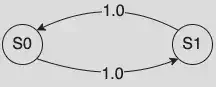
Particularly, this chain has a period 2.

Summarise in a diagram