In this section we ask what values measurements on normal, healthy people are likely to have. There are difficulties in doing this. Who is `normal' anyway? In the UK population almost everyone has hard fatty deposits in their coronary arteries, which result in death for many of them. Very few Africans have this; they die from other causes. So it is normal in the UK to have an abnormality. We usually say that normal people are the apparently healthy members of the local population. We can draw a sample of these as described in Chapter 3 and make the measurement on them.
The next problem is to estimate the set of values. If we use the range of the observations, the difference between the two most extreme values, we can be fairly confident that if we carry on sampling we will eventually find observations outside it, and the range will get bigger and bigger (Section 4.7). To avoid this we use a range between two quantiles (Section 4.7), usually the 2.5 centile and the 97.5 centile, which is called the normal range, 95% reference range, or 95% reference interval. This leaves 5% of normals outside the `normal range', which is the set of values within which 95% of measurements from apparently healthy individuals will lie.
A third difficulty comes from confusion between `normal' as used in medicine and `Normal distribution' as used in statistics. This has led some people to develop approaches which say that all data which do not fit under a Normal curve are abnormal! Such methods are simply absurd, there is no reason to suppose that all variables follow a Normal distribution (Section 7.4, Section 7.5). The term `reference interval', which is becoming widely used, has the advantage of avoiding this confusion. However, the most commonly used method of calculation rests on the assumption that the variable follows a Normal distribution.
We have already seen that in general most observations fall within two standard deviations of the mean, and that for a Normal distribution 95% are within these limits with 2.5% below and 2.5% above. If we estimate the mean, m, and standard deviation, s, of data from a Normal population we can estimate the reference interval as m - 2s to m + 2s.
The following data are the Forced Expiratory Volume (litres) in one second (FEV1) for 57 male medical stdents:
2.85  3.19  3.50  3.69  3.90  4.14  4.32  4.50  4.80  5.20
2.85  3.20  3.54  3.70  3.96  4.16  4.44  4.56  4.80  5.30
2.98  3.30  3.54  3.70  4.05  4.20  4.47  4.68  4.90  5.43
3.04  3.39  3.57  3.75  4.08  4.20  4.47  4.70  5.00
3.10  3.42  3.60  3.78  4.10  4.30  4.47  4.71  5.10
3.10  3.48  3.60  3.83  4.14  4.30  4.50  4.78  5.10
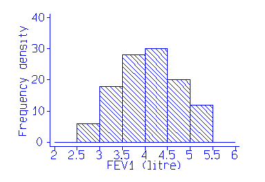
We will estimate the reference interval for FEV1 in male medical students. The data seem to follow a Normal distriibution reasonably well:

We have 57 observations, mean 4.06 and standard deviation 0.67 litres. The reference interval is thus 2.7 to 5.4 litres. From Table 4.4 we see that in fact only one student (2%) is outside these limits, although the sample is rather small.
As the observations are assumed to be from a Normal distribution, standard
errors and confidence intervals for these limits are easy to find. The
estimates m and s are independent (Section 7A) with variances
s2/n
and s2/2(n -1)} (Section 8.2, Section 8.7). The
sample mean m follows a Normal distribution and
s a distribution
which is approximately Normal. Hence m - 2s is from a Normal
distribution with variance:
VAR(m - 2s) = VAR(m) + VAR(2s)
= VAR(m) + 4VAR(s)
= s2/n + 4s2/2(n
- 1)
= s2(1/n + 2/(n - 1))
Hence, provided Normal assumptions hold, the standard error of the
limit of the reference interval is
root (s2(1/n + 2/(n - 1)))
If n is large, this is approximately
root (3s2/n).
For the FEV1 data, this is the square root of 3 * 0.67 2/57 = 0.15. Hence the 95% confidence intervals for these limits are 2.7 +/- 1.96 times 0.15 and 5.4 +/- 1.96 times 0.15, i.e. from 2.4 to 3.0 and 5.1 to 5.7 litres.
Compare the following data, serum triglyceride measurements in cord blood from 282 babies:
0.15  0.29  0.34  0.38  0.41  0.46  0.52  0.56  0.64  0.80
0.16  0.30  0.34  0.38  0.41  0.46  0.52  0.56  0.64  0.80
0.20  0.30  0.34  0.38  0.41  0.46  0.52  0.56  0.65  0.82
0.20  0.30  0.34  0.39  0.42  0.46  0.52  0.57  0.66  0.82
0.20  0.30  0.34  0.39  0.42  0.47  0.52  0.57  0.66  0.82
0.20  0.30  0.34  0.39  0.42  0.47  0.52  0.58  0.66  0.82
0.21  0.30  0.34  0.39  0.42  0.47  0.52  0.58  0.66  0.83
0.22  0.30  0.35  0.39  0.42  0.47  0.53  0.58  0.66  0.84
0.24  0.30  0.35  0.40  0.42  0.47  0.54  0.58  0.67  0.84
0.25  0.30  0.35  0.40  0.44  0.48  0.54  0.59  0.67  0.84
0.26  0.31  0.35  0.40  0.44  0.48  0.54  0.59  0.68  0.86
0.26  0.31  0.35  0.40  0.44  0.48  0.54  0.59  0.70  0.87
0.26  0.32  0.35  0.40  0.44  0.48  0.54  0.59  0.70  0.88
0.27  0.32  0.36  0.40  0.44  0.48  0.54  0.60  0.70  0.88
0.27  0.32  0.36  0.40  0.44  0.48  0.55  0.60  0.70  0.95
0.27  0.32  0.36  0.40  0.44  0.48  0.55  0.60  0.72  0.96
0.28  0.32  0.36  0.40  0.44  0.48  0.55  0.60  0.72  0.96
0.28  0.32  0.36  0.40  0.44  0.48  0.55  0.60  0.74  0.99
0.28  0.32  0.36  0.40  0.45  0.48  0.55  0.60  0.75  1.01
0.28  0.32  0.36  0.40  0.45  0.48  0.55  0.60  0.75  1.02
0.28  0.33  0.36  0.40  0.45  0.48  0.55  0.60  0.76  1.02
0.28  0.33  0.36  0.40  0.45  0.49  0.55  0.61  0.76  1.04
0.28  0.33  0.37  0.40  0.45  0.49  0.56  0.62  0.78  1.08
0.28  0.33  0.37  0.40  0.45  0.49  0.56  0.62  0.78  1.11
0.29  0.33  0.37  0.41  0.46  0.50  0.56  0.63  0.78  1.20
0.29  0.33  0.37  0.41  0.46  0.50  0.56  0.64  0.78  1.28
0.29  0.33  0.38  0.41  0.46  0.50  0.56  0.64  0.78  1.64
0.29  0.33  0.38  0.41  0.46  0.50  0.56  0.64  0.78  1.66
0.29  0.34
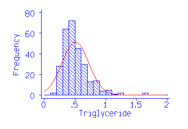
As already noted (Sections 4.4 and 7.4), the data are highly skewed:

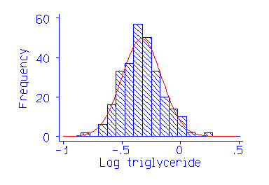
The log transformed data give a breathtakingly symmetrical distribution:

Because of the obviously unsatisfactory nature of the Normal method for some data, some authors have advocated the estimation of the percentiles directly (Section 4.5, Medians and quantiles ), without any distributional assumptions. This is an attractive idea. We want to know the point below which 2.5% of values will fall. Let us simply rank the observations and find the point below which 2.5% of the observations fall. For the 282 triglycerides, the 2.5 and 97.5 centiles are found as follows. For the 2.5 centile, we find i = q(n + 1) = 0.025 * (282 +1) = 7.08. The required quantile will be between the 7th and 8th observation. The 7th is 0.21, the 8th is 0.22 so the 2.5 centile would be estimated by 0.21 + (0.22 - 0.21) * (7.08 - 7) = 0.211. Similarly the 97.5 centile is 1.039.
This approach gives an unbiased estimate whatever the distribution.
The log transformed triglyceride would give exactly the same results. Note
that the Normal theory limits from the log transformed data are very similar.
We now look at the confidence interval. The 95% confidence interval for
the q quantile, here q being 0.025 or 0.975, estimated directly
from the data is found by the Binomial distribution method (Section
8.9). For the triglyceride data, n = 282 and so for the lower
limit, q = 0.025, we have
j = 282 * 0.025 - 1.96 root (282 * 0.025 * 0.975)
k = 282 * 0.025 + 1.96 root (282 * 0.025 * 0.975)
This gives j = 1.9 and k = 12.2, which we round up to
j
= 2 and k = 13. In the triglyceride data the second observation,
corresponding to j= 2, is 0.16 and the 13th is 0.26. Thus the 95%
confidence interval for the lower reference limit is 0.16 to 0.26. The
corresponding calculation for q = 0.975 gives j = 270 and
k
= 281. The 270th observation is 0.96 and the 281st is 1.64, giving a 95%
confidence interval for the upper reference limit of 0.96 to 1.64. These
are wider confidence intervals than those found by the Normal method, those
for the long tail particularly so. This method of estimating percentiles
in long tails is relatively imprecise.
Back to An Introduction to Medical Statistics contents
Back to Martin Bland's Home Page
This page maintained by Martin Bland
Last updated: 10 November, 2003