Extract from An Introduction to Medical Statistics
by Martin Bland
This is a section from my text book An Introduction to Medical Statistics,
Fourth Edition. I hope that the topic will be useful in its own right,
as well as giving a flavour of the book. Section references are to the
book.
10.7 Serial data
Table 10.5 shows levels of zidovudine (AZT)
in the blood of AIDS patients
at several times after administration of the drug, for patients with normal
fat absorption or fat malabsorption.
Table 10.5 Blood zidovudine levels at times after administration of the drug by presence of fat malabsorption (data from
Kapembwa et al. 1996)
Malabsorption patients:
            Time since administration of zidovudine (min)
 0     15    30    45    60    90   120   150   180   240   300   360
0.08 13.15  5.70  3.22  2.69  1.91  1.72  1.22  1.15  0.71  0.43  0.32
0.08  0.08  0.14  2.10  6.37  4.89  2.11  1.40  1.42  0.72  0.39  0.28
0.08  0.08  3.29  3.47  1.42  1.61  1.41  1.09  0.49  0.20  0.17  0.11
0.08  0.08  1.33  1.71  3.30  1.81  1.16  0.69  0.63  0.36  0.22  0.12
0.08  6.69  8.27  5.02  3.98  1.90  1.24  1.01  0.78  0.52  0.41  0.42
0.08  4.28  4.92  1.22  1.17  0.88  0.34  0.24  0.37  0.09  0.08  0.08
0.08  0.13  9.29  6.03  3.65  2.32  1.25  1.02  0.70  0.43  0.21  0.18
0.08  0.64  1.19  1.65  2.37  2.07  2.54  1.34  0.93  0.64  0.30  0.20
0.08  2.39  3.53  6.28  2.61  2.29  2.23  1.97  0.73  0.41  0.15  0.08

Normal absorption patients:
            Time since administration of zidovudine (min)
 0     15    30    45    60    90   120   150   180   240   300   360
0.08  3.72 16.02  8.17  5.21  4.84  2.12  1.50  1.18  0.72  0.41  0.29
0.08  6.72  5.48  4.84  2.30  1.95  1.46  1.49  1.34  0.77  0.50  0.28
0.08  9.98  7.28  3.46  2.42  1.69  0.70  0.76  0.47  0.18  0.08  0.08
0.08  1.12  7.27  3.77  2.97  1.78  1.27  0.99  0.83  0.57  0.38  0.25
0.08 13.37 17.61  3.90  5.53  7.17  5.16  3.84  2.51  1.31  0.70  0.37
A line graph of these data was shown in
Figure 5.11.
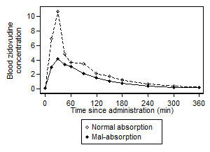
Figure 5.11 Line graph to show the response to
administration of zidovudine in two groups of AIDS patients
(data from Kapembwa et al. 1996).
One common approach to such data is to carry out a two sample t test
at each time separately, and researchers often ask at what time the difference
becomes significant. This is a misleading question, as significance is
a property of the sample rather than the population. The difference at
15 minutes may not be significant because the sample is small and the difference
to be detected is small, not because there is no difference in the population.
Further, if we do this for each time point we are carrying out multiple
significance tests (Section 9.10) and each test
only uses a small part of the data so we are losing power (Section 9.9).
It is better to ask whether there is any evidence of a difference between
the response of normal and malabsorption subjects over the whole period
of observation.
The simplest approach is to reduce the data for a subject to one number.
We can use the highest value attained by the subject, the time at which
this peak value was reached, or the area under the curve. The first two
are self-explanatory. The area under the curve or AUC is
found by drawing a line through all the points and finding the area between
it and the horizontal axis. The ‘curve’ is ususally formed by a series
of straight lines found by joining all the points for the subject,
and Figure 10.10 shows this
for the first participant in Table 10.5.
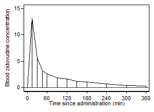
Figure 10.10 Calculation of the area under the curve for
one subject (data supplied by Moses Kapembwa, personal
communication).
The area under the curve can be calculated by taking each straight line
segment and calculating the area under this. This is the base multiplied
by the average of the two vertical heights. We calculate this for each
line segment, i.e. between each pair of adjacent time points, and add.
Thus for the first subject we get
(15 − 0) × (0.08 + 13.15)/2 + (30 − 15 )
× ( 13.15 + 5.70 )/2
+ ... + (360 − 300) × (0.43 + 0.32)/2 = 667.425.
This can be done fairly easily by most statistical computer packages.
The area for each subject is shown in Table 10.6.
Table 10.6 Area under the curve for data of Table 10.5 (data
from Kapembwa et al. 1996)
Malabsorption                  Normal
patients                       patients
------------------             --------
667.425    256.275              919.875
569.625    527.475              599.850
306.000    388.800              499.500
298.200    505.875              472.875
617.850                        1377.975
We can now compare the mean area by the two sample t method.
As Figures 10.11 and
10.12 show,
the log area gives a better fit to the Normal distribution
than does the area itself.
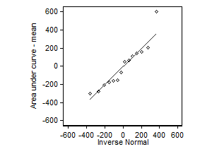
Figure 10.11 Normal plot for area under the curve for the
data of Table 10.5 (data supplied by Moses Kapembwa,
personal communication).
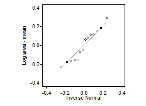 Figure 10.12 Normal plot for log area under the curve for
the data of Table 10.5 (data supplied by Moses Kapembwa,
personal communication).
Figure 10.12 Normal plot for log area under the curve for
the data of Table 10.5 (data supplied by Moses Kapembwa,
personal communication).
Using the log area we get n1 = 9, mean1 = 2.639541,
s1 = 0.153376 for malabsorption subjects and n2=5
, mean2 = 2.850859, s2 = 0.197120 for the normal
subjects. The common variance is s2 = 0.028635, standard error
of the difference between the means is square root of 0.028635 × (1/9+1/5),
which gives 0.094385, and the t statistic is t = (2.639541 − 2.850859)/0.094385
= −2.24 which has 12 degrees of freedom, P = 0.04. The 95% confidence interval
for the difference is 2.639541 − 2.850859 +/− 2.18 times 0.094385, giving
−0.417078 to −0.005558, and if we antilog this we get 0.38 to 0.99. Thus
the area under the curve for malabsorption subjects is between 0.38 and
0.99 of that for normal AIDS patients, and we conclude that malabsorption
inhibits uptake of the drug by this route. A fuller discussion of the analysis
of serial data is given by Matthews et al. (1990).
References
Matthews, J.N.S., Altman, D.G., Campbell, M.J., and Royston, P. (1990)
Analysis of serial measurements in medical research. British Medical
Journal 300 230-35.
Adapted from pages 142–144 of
An Introduction to Medical Statistics by Martin Bland, 2015,
reproduced by permission of
Oxford University Press.
Back to An Introduction to Medical Statistics
contents
Back to Martin Bland’s Home Page
This page maintained by Martin Bland.
Last updated: 7 August, 2015
Back to top