The simple 95% limits of agreement method relies on the assumptions that the mean and standard deviation of the differences are constant, i.e. that they do not depend on the magnitude of the measurement. In our original papers, we desribed the common situation where the standard deviation is proportional to the magnitude and described a method using a logarithmic transformation of the data. In our 1999 review paper (Bland and Altman 1999) we described a method for dealing with any relationship between mean and SD of differences and the magnitude of the measurement. (This was Doug Altman's idea, I can take no credit.)
In this note I shall illustrate it with some measurements of blood glucose using capillary (i.e. finger-prick) blood measured on the spot, and plasma gluose measured from a venous blood sample taken to the laboratory.
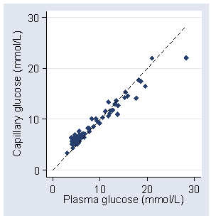
We have 88 measurements of capillary and plasma glucose (Martin et al., 2005). A scatter diagram with the line of equality shows a clear trend in the bias, being positive (i.e. capillary glucose higher) for small glucose measures and negative for high glucose measures.

The plot of difference against the average of the two glucose measurements shows this even more clearly:
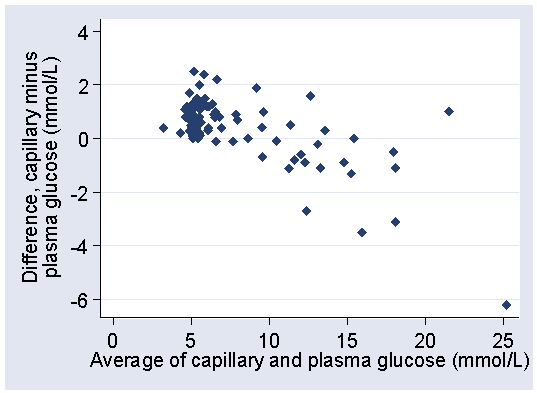
The differences tend to be positive when glucose is low, negative when glucose is high.
If we estimate the crude 95% limits of agreement ignoring this relationship, we have mean difference = 0.3625 mmol/L, SD = 1.2357 mmol/L
crude lower limit = 0.3625 − 1.96 × 1.2357 = −2.06 mmol/L
crude upper limit = 0.3625 + 1.96 × 1.2357 = 2.78 mmol/L
Plotting these on the difference versus mean plot:
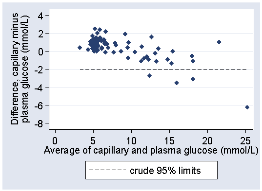
we can see that the limits do not fit the data well. They are too wide at the low glucose end and too narrow at the high glucose end. They are correct in that they are expected to include 95% of differences (here 84/88 = 94.5%) but all the differences outside the limits are at one end and one of them is a long way outside.
A better fit can be found by using a regression method (Bland and Altman 1999). Regression of difference on average gives a highly significant relationship, P<0.001:
difference = 1.8799 − 0.1943 × average glucose
We can use this to model the relationship between mean difference and the magnitude of the blood glucose. If we take the residuals about this line, the differences between the observed difference and the difference predicted by the regression, we can use these to model the relationship between the standard deviation of the differences and the magnitude of the blood glucose. We calculate the absolute values of the residuals, without sign, and then do regression of these on the average glucose. This gives the following regression equation:
absolute residual = −0.02887 + 0.08525 × average glucose
which is statistically significant (P<0.001). If we multiply these coefficients by the square root of (pi over 2) we get an equation to predict the standard deviation of the differences:
SD = −0.03618 + 0.1068 × average glucose
This is because the mean of the absolute value a Standard Normal distribution is root(2/pi) and the mean of the absolute value of a Normal distribution with mean zero and standard deviation sigma is root (2 / pi) sigma.
If we predict mean difference and standard deviation from these equations, we can estimate mean minus or plus 1.96 SD for any magnitude of glucose:
lower limit = 1.8799 − 0.1943 × average glucose − 1.96 × (−0.03618 + 0.1068 × average glucose)
= 1.8799 − 1.96 × (−0.03618) +(−0.1943 − 1.96 × 0.1068) × average glucose
= 1.9508 − 0.4036 × average glucose
Similarly,
upper limit = 1.8799 + 1.96 × (−0.03618) +(−0.1943 + 1.96 × 0.1068) × average glucose
= 1.8090 + 0.0150 × average glucose
We can plot these limits on the difference versus mean plot:
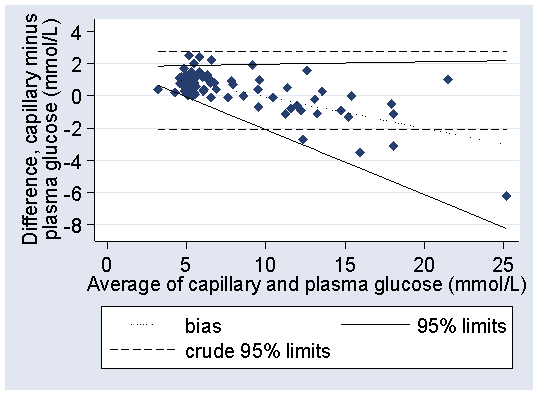
The fit is greatly improved, particularly at the high glucose end. In practice, it would be sufficient to round these considerably, to between 2.0 − 0.4 × glucose and +1.8 mmol/L
This used linear fits, but we could consider the possibility that the relationship are not linear. For example, we can add an average squared term to the regression of difference on average:
difference = 1.5190 − 0.1274 × glucose − 0.008662 × (glucose − 7.8)2
(7.8 mmol/L is the mean average glucose and is subtracted to make the glucose and glucose squared terms uncorrelated.) The squared term is statistically significant (P=0.03). We can calculate the absolute residuals for this model and regress them on the average glucose, as before:
absolute residual = −0.03165 + 0.08221 × average glucose
Multiplying by the square root of (2 over pi) gives
SD = −0.3967 + 0.1030 × average glucose
We could use these regression equations to the estimate the 95% limits of agreement, as before:
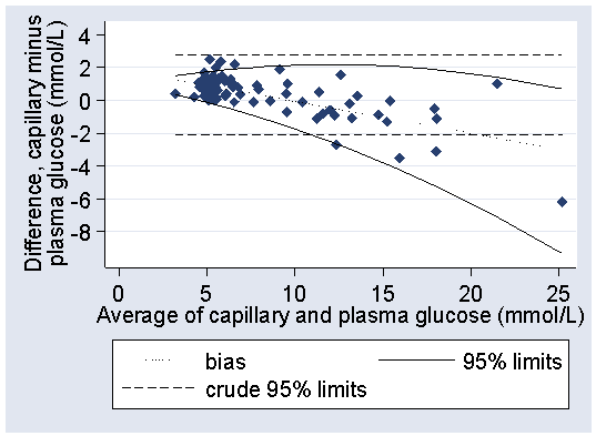
Despite the improved fit to the data, the increased difficulty of using curved limits makes the linear limits, 2.0 − 0.4 × glucose to 1.8 mmol/L, a more practical estimate for the 95% limits for the difference between capillary and plasma glucose in this population.
I thank Max Bulsara and David Martin for generously supplying their data. I also thank Ernesto Ramirez for pointing out an error on the page.
Bland JM, Altman DG. (1999) Measuring agreement in method comparison studies. Statistical Methods in Medical Research 8, 135-160.
Martin DD, Shephard MDS, Freeman H, Bulsara MK, Jones TW, Davis EA, Maguire GP. (2005) Point-of-care testing of HbA(1c) and blood glucose in a remote Aboriginal Australian community. Medical Journal of Australia 182: 524-527.
Back to measurement studies menu.
Back to Martin Bland's home page.
To Douglas Altman's home page.
This page maintained by Martin Bland.
Last updated: 10 December, 2009.