Allocation by minimisation
(This section is based on Bland et al., Statistics Guide for Research Grant Applicants. I am grateful to Sally Kerry for the example.)
In small studies with several important prognostic variables, random allocation may not provide adequate balance in the groups. Stratified allocation may not be feasible due to there being too few subjects to stratify by all important variables. It may be possible to achieve balance by minimisation.
Minimisation is based on the idea that the next patient to enter the trial is given whichever treatment would minimise the overall imbalance between the groups at that stage of the trial.
I shall explain this using an example, a cluster randomised trial in general practice, where 16 general practices were to be allocated to intervention and control groups.
There were three variables on which the groups should be balanced:
- number of doctors in the practice,
- number of patients in the practice,
- number of long-term mentally ill patients.
We first classify these minimisation variables into convenient groups, aiming for a roughly equal split if possible:
- number of doctors in the practice: 3 or 4 vs. 5 or 6,
- number of patients in the practice: <8,600 vs. ≥8.600,
- number of long-term mentally ill patients: <25 vs. ≥25.
The first practice had:
- number of doctors: 4,
- number of patients: 8,500,
- number of long-term mentally ill: 23.
The two treatment groups were perfectly balanced at the outset, being empty, so there was no reason to choose either group for the first practice. This practice was therefore allocated randomly. It was allocated to Intervention.
This gives the following table for the minimisation variables:
| Intervention | Control | |
|---|---|---|
| 3 or 4 doctors | 1 | 0 |
| 5 or 6 doctors | 0 | 0 |
| <8,600 patients | 1 | 0 |
| ≥8.600 patients | 0 | 0 |
| <25 mentally ill | 1 | 0 |
| ≥25 mentally ill | 0 | 0 |
The second practice had number of doctors = 4, number of patients = 7,800, number of long-term mentally ill = 17.
The second practice would affect the highlighted rows:
| Intervention | Control | |
|---|---|---|
| 3 or 4 doctors | 1 | 0 |
| 5 or 6 doctors | 0 | 0 |
| <8,600 patients | 1 | 0 |
| ≥8.600 patients | 0 | 0 |
| <25 mentally ill | 1 | 0 |
| ≥25 mentally ill | 0 | 0 |
| Imbalance | 3 | 0 |
If we were to allocate the second practice to Intervention, we would have imbalance 6 and 0, if we were to allocate to Control we would have 3 and 3. Hence we allocate the second practice to Control. This gave the following table for the minimisation variables:
| Intervention | Control | |
|---|---|---|
| 3 or 4 doctors | 1 | 1 |
| 5 or 6 doctors | 0 | 0 |
| <8,600 patients | 1 | 1 |
| ≥8.600 patients | 0 | 0 |
| <25 mentally ill | 1 | 1 |
| ≥25 mentally ill | 0 | 0 |
The third practice had number of doctors = 5, number of patients = 10,000, number of long-term mentally ill = 24.
The third practice would affect the highlighted rows:
| Intervention | Control | |
|---|---|---|
| 3 or 4 doctors | 1 | 1 |
| 5 or 6 doctors | 0 | 0 |
| <8,600 patients | 1 | 1 |
| ≥8.600 patients | 0 | 0 |
| <25 mentally ill | 1 | 1 |
| ≥25 mentally ill | 0 | 0 |
| Imbalance | 1 | 1 |
The groups were now perfectly balanced, so the balance would be the same whichever group the third practice went into. The third practice was allocated randomly. It was allocated to intervention. This gave the following table for the minimisation variables:
| Intervention | Control | |
|---|---|---|
| 3 or 4 doctors | 1 | 1 |
| 5 or 6 doctors | 1 | 0 |
| <8,600 patients | 1 | 1 |
| ≥8.600 patients | 1 | 0 |
| <25 mentally ill | 2 | 1 |
| ≥25 mentally ill | 0 | 0 |
The fourth practice had number of doctors = 3, number of patients = 3,400, number of long-term mentally ill = 12.
The fourth practice would affect the highlighted rows:
| Intervention | Control | |
|---|---|---|
| 3 or 4 doctors | 1 | 1 |
| 5 or 6 doctors | 1 | 0 |
| <8,600 patients | 1 | 1 |
| ≥8.600 patients | 1 | 0 |
| <25 mentally ill | 2 | 1 |
| ≥25 mentally ill | 0 | 0 |
| Imbalance | 4 | 3 |
To minimise the imbalance, we allocate to Control.
The fourth practice was allocated to Control, giving the following table:
| Intervention | Control | |
|---|---|---|
| 3 or 4 doctors | 1 | 2 |
| 5 or 6 doctors | 1 | 0 |
| <8,600 patients | 1 | 2 |
| ≥8.600 patients | 1 | 0 |
| <25 mentally ill | 2 | 2 |
| ≥25 mentally ill | 0 | 0 |
The allocation continued in this way, each practice being allocated so as to minimise the imbalance between the treatment groups. After all 16 practices, the minimisation table looked like this:
| Intervention | Control | |
|---|---|---|
| 3 or 4 doctors | 5 | 5 |
| 5 or 6 doctors | 3 | 3 |
| <8,600 patients | 4 | 4 |
| ≥8.600 patients | 4 | 4 |
| <25 mentally ill | 4 | 4 |
| ≥25 mentally ill | 4 | 4 |
The trial was perfectly balanced.
There are some problems with minimisation:
- Minimisation is not random. Groups may not be balanced on characteristics not minimised for.
- The Food and Drugs Administration does not accept it.
- It may be possible for the patient's characteristics to influence the investigator's decision about recruiting that patient to the trial, the investigator might know what treatment the patient would receive.
We can introduce an element of randomisation into minimisation. We use the minimisation method to decide in which direction the subject should be allocated, but use unequal randomisation to choose the actual treatment. For example, we might allocate in favour of the allocation which would reduce imbalance with probability 2/3 or 3/4, and in the direction which would increase imbalance with probability 1/3 or 1/4.
In the GP practice allocation above, the first practice was allocated randomly anyway.
The second practice had number of doctors = 4, number of patients = 7,800, number of long-term mentally ill = 17.
The minimisation table was:
| Intervention | Control | |
|---|---|---|
| 3 or 4 doctors | 1 | 0 |
| 5 or 6 doctors | 0 | 0 |
| <8,600 patients | 1 | 0 |
| ≥8.600 patients | 0 | 0 |
| <25 mentally ill | 1 | 0 |
| ≥25 mentally ill | 0 | 0 |
| Imbalance | 3 | 0 |
This indicates that allocation to control would reduce the imbalance. We therefore made a random choice with probability 1 in 4 for Intervention and 3 in 4 for Control. My choice was (1 in 4): Intervention
The third practice had number of doctors = 5, number of patients = 10,000, number of long-term mentally ill = 24.
The imbalance would be:
| Intervention | Control | |
|---|---|---|
| 3 or 4 doctors | 2 | 0 |
| 5 or 6 doctors | 0 | 0 |
| <8,600 patients | 2 | 0 |
| ≥8.600 patients | 0 | 0 |
| <25 mentally ill | 2 | 0 |
| ≥25 mentally ill | 0 | 0 |
| Imbalance | 2 | 0 |
The fourth practice had number of doctors = 3, number of patients = 3,400, number of long-term mentally ill = 12.
The imbalance would be:
| Intervention | Control | |
|---|---|---|
| or 4 doctors | 2 | 0 |
| 5 or 6 doctors | 0 | 1 |
| <8,600 patients | 2 | 0 |
| ≥8.600 patients | 0 | 1 |
| <25 mentally ill | 2 | 1 |
| ≥25 mentally ill | 0 | 0 |
| Imbalance | 6 | 1 |
Control was indicated and the random choice (3 in 4) was allocation to Control. This gave us the following table:
| Intervention | Control | |
|---|---|---|
| 3 or 4 doctors | 2 | 1 |
| 5 or 6 doctors | 0 | 1 |
| <8,600 patients | 2 | 1 |
| ≥8.600 patients | 0 | 1 |
| <25 mentally ill | 2 | 2 |
| ≥25 mentally ill | 0 | 0 |
And so on . . .
Minimisation is most useful when a small and variable group must be randomised. Large samples will be balanced after ordinary randomisation or can be stratified. Variables which are used in minimisation or stratification should be taken into account in the analysis if possible, as this will reduce the variability within the groups. We do not need to do minimisation by hand, there are programs and central randomisation services which will do it for us.
In a factorial trial, we have more than one treatment choice. Participants are randomised more than once. We can do this either to get two trials for price of one or to estimate the possible interaction between the two treatments.
For example, Peveler et al. (1999) looked at the effect of antidepressant drug counselling and information leaflets on adherence to drug treatment in primary care patients with depression.
Patients were randomised to four groups:
- counselling and leaflet
- counselling
- leaflet
- neither
The results were as follows:
| Leaflet | Drug counselling | Total | |
|---|---|---|---|
| Yes | No | ||
| Yes | 34/52 (65%) | 22/53 (42%) | 56/105 (53%) |
| No | 32/53 (60%) | 20/55 (36%) | 52/108 (48%) |
| Total | 66/105 (63%) | 42/108 (39%) | |
From this table, we can estimate the effects of counselling and the effects of the leaflet. We can carry out a test of significance for each. Counselling has a highly significant effect, P=0.001. The leaflet does not have a significant effect, P=0.4. For these tests and associated estimates, the effect of each treatment must not be influenced by the presence of the other. In statistics, we say there is no interaction between counselling and leaflet in their effects on adherence.
In this case, there is nothing to suggest an interaction:
| Leaflet | Drug counselling | Total | |
|---|---|---|---|
| Yes | No | ||
| Yes | 65% | 42% | 53% |
| No | 60% | 36% | 48% |
| Total | 63% | 39% | |
The effect of counselling is the same whether the leaflet was given or not and the effect of the leaflet is the same whether the counselling was given or not. We can carry out a significance test for the presence of an interaction. In this example: P = 0.99, so there is indeed no evidence for one.
This is a hypothetical table showing a positive interaction:
| Leaflet | Drug counselling | Total | |
|---|---|---|---|
| Yes | No | ||
| Yes | 95% | 42% | 53% |
| No | 60% | 36% | 48% |
| Total | 63% | 39% | |
Here the effect of counselling is greater when leaflet is given than when it is not. Looking at it another way, the effect of the leaflet is greater when counselling is given than when it is not. (These are completely hypothetical data, please do not remember them as an example of counselling research!) The effect of two treatments working together like this, each being more effective when the other is applied, is sometimes called synergy.
This is a hypothetical table showing a negative interaction:
| Leaflet | Drug counselling | Total | |
|---|---|---|---|
| Yes | No | ||
| Yes | 65% | 60% | 53% |
| No | 60% | 36% | 48% |
| Total | 63% | 39% | |
In this table, the effect of counselling is less when leaflet is given than when it is not. This can happen when there is a ceiling effect. The compliance can be improved by either treatment, but not beyond a limit. (Again, these are not real, but hypothetical, data.)
Detecting interactions requires large sample sizes, much larger than are required to detect the simple treatment effect. This is because we usually get a smaller difference between the effects of a treatment in the presence or absence of the other treatment than we do between the presence of absence of the first treatment.
We can have any number of factors, not restricted to two. For example, Dale et al. (1999) carried out three different treatment comparisons in a trial of the treatment of venous leg ulcers:
- drug — pentoxifylline 400 mg three times daily or matching placebo,
- dressing — knitted viscose dressing or a hydrocolloid dressing,
- compression — elastic single layer compression or a four layer bandaging regimen.
There are 2×2×2 = 8 treatment groups altogether.
Back to top.
Sequential clinical trials
In clinical trials, data are usually accumulated over a long period. Why do we have to wait until the end of the trial to see the data and analyse them? Why not analyse the data as we go along and stop the trial when we have a significant treatment difference?
If we were to carry out sequential tests like this using the usual statistical methods such as t and chi-squared tests, we will be misled. Multiple testing will make the P values far too small. For example, if we carry out repeated t test at alpha = 0.05 where the null hypothesis is true, the probability of a "significant" difference = 0.39, not 0.05.
We must use special sequential tests to give a true P value. There are many ways of doing this. In all of them, we calculate the value of the difference which would have to be exceeded for each sample size, such that if we stop the trial when this is exceeded the P value will be 0.05.
As for the sample size of a fixed trial, this value depends on the difference we are looking for, the variability, the power, and alpha. The following example of a sequential test was given by Whitehead (1997). It concerns a trial of two types of anaesthesia for outpatient abortion. The outcome variable was the report of serious nausea, yes or no. The expected control proportion was 20% and the difference to be detected was 15 percentage points, i.e. down to 5%. This is a pretty big difference. The chosen power was 90% and the significance level alpha was 5%.
A fixed sample size trial would require 200 patients in total.
Suppose after nE patients on the experimental treatment and nC control patients we have observed SE and SC successes (no nausea), a total of S successes and F failures out of n subjects.
Define the efficient score

and the Fisher information

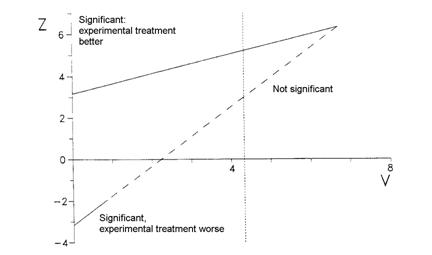
We use a graphical presentation of the test and plot Z against V as data accumulate. Whitehead used a triangular testing scheme, mainly aimed at detecting improvement with the experimental treatment. The data are plotted on the following test template:
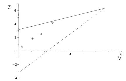
These were the results of the anaesthesia trial:
| Date | Experimental treatment | Control treatment | Z | V | ||||
|---|---|---|---|---|---|---|---|---|
| SE | FE | nE | SC | FC | nC | |||
| 5 January | 8 | 0 | 8 | 6 | 1 | 7 | 0.57 | 0.25 |
| 2 February | 21 | 1 | 22 | 13 | 4 | 17 | 2.09 | 1.23 |
| 2 March | 33 | 2 | 35 | 21 | 6 | 27 | 2.89 | 1.97 |
| 30 March | 38 | 3 | 41 | 23 | 10 | 33 | 4.71 | 2.97 |
The values of Z and V were calculated on each date and plotted on the testing template:
This template assumes that the values of Z and V are calculated every time a participant goes into the trial and plotted on the testing template. We can adjust the template for taking only a few looks, as was done in this trial:
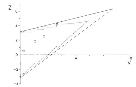
This is called a Christmas tree boundary, for obvious reasons.
This trial reached the boundary after 74 participants had been recruited. A fixed sample size trial would have recruited 200 participants before the analysis was carried out. Hence this trial was very efficient.
However, if the trial had carried on until the top right corner of the template had been reached, the maximum number of participants who might have been recruited is is 890 for testing after every participant. Using the Christmas tree boundary, the maximum patients who might be recruited is 650.
We trade off the high probability of a shorter trial against the low probability of a longer trial.
Sequential trials have several advantages over fixed sample size designs:
- they are usually quicker and hence cheaper,
- expose fewer patients to untested treatments, especially if unsafe.
They have some disadvantages, too:
- they may last longer if treatment benefits are small,
- they are technically complex,
- the confidence interval for the treatment effect may be wide (but excluding zero).
The Key reference text is John Whitehead's The Design and Analysis of Sequential Clinical Trials, revised 2nd. ed. Warning: this is a highly technical book most suitable for statisticians.
John Whitehead also has software to enable you to carry out sequential designs: PEST 4 http://www.maths.lancs.ac.uk/department/research/statistics/mps/pest.
The last time I looked, the current price was £2,000 to industry, academic price £1,000. I would not think of doing such a trial without it.
Bland JM, Butland BK, Peacock JL, Poloniecki J, Reid F, Sedgwick P. Statistics Guide for Research Grant Applicants . London: St. George's Hospital Medical School.
Dale JJ, Ruckley CV, Harper DR, Gibson B, Nelson EA, Prescott RJ. (1999) Randomised, double blind placebo controlled trial of pentoxifylline in the treatment of venous leg ulcers. British Medical Journal 319: 875-878.
Peveler R, George C, Kinmonth A-L, Campbell M, Thompson C. (1999) Effect of antidepressant drug counselling and information leaflets on adherence to drug treatment in primary care: randomised controlled trial. British Medical Journal 319: 612-615.
Whitehead J. The Design and Analysis of Sequential Clinical Trials, revised 2nd. ed. Wiley: Chichester, 1997.
To Martin Bland's M.Sc. index.
This page maintained by Martin Bland.
Last updated: 20 July, 2009.