Cross-over trials

• What is a cross-over trial?
• Advantages of cross-over designs
• Estimation and significance tests
• Analysis for a simple two period two treatment crossover trial
• Interaction between period and treatment
• Carry over effects
• Should we test the period × treatment interaction?
• Washout periods
• Baseline measurements
• Books on cross-over trials
• References

In these notes I shall describe the uses of and contra-indications for cross-over trials, the analysis of a cross-over trial comparing two treatments, and some features of cross-over trial design. I shall be describing a recent trial on which I have collaborated and two older trials drawn from the literature.

For example, an early two treatment cross-over trial was done to compare pronethalol with placebo for the treatment of angina pectoris. Patients received placebo for two periods of two weeks and pronethalol for two periods of two weeks, in random order (Pritchard et al. 1963). They completed diaries of attacks of angina. The results were as follows:

Attacks of angina recorded over four weeks:

Placebo:	2	3	7	8	14	17
	23	34	60	79	71	323
Pronethalol:	0	0	1	2	7	15
	16	25	29	41	65	348

There is great variability in the numbers of attacks and the difference is not significant. The Mann Whitney U test gives P = 0.4. But this analysis is wrong; it ignores the data structure. These observations should be paired, as in Table 1.

Table 1. Results of a trial of pronethalol for the treatment of angina pectoris (Pritchard et al., 1963)

Patient	Placebo	Pronethalol	Placebo minus   Pronethalol
1	71	29	42
2	323	348	–25
3	8	1	7
4	14	7	7
5	23	16	7
6	34	25	9
7	79	65	14
8	60	41	19
9	2	0	2
10	3	0	3
11	17	15	2
12	7	2	5

Now we can see, despite the great variability, a suggestion of a treatment effect. Eleven of the 12 participants had more attacks on placebo than on pronethalol. As the distribution of differences in far from Normal, we can use the sign test to compare the two treatments. This gives P = 0.006. We have a highly significant difference compared to that for a two sample analysis using the Mann Whitney U test, which gave P = 0.4.

Back to top.

Advantages of cross-over designs

Cross-over designs have several advantages over a parallel group design of the same size:

• each participant acts as their own control,
• removes variability between participants,
• fewer subjects needed.

They have some disadvantages, too:

• short term treatment, because we need to switch treatments before participants quit the trial,
• no follow-up, because at the end of treatment all patients have had both treatments.

Cross-over trials are not suitable for many disease and treatment combinations. Cross-over trials are suitable for:

• chronic diseases (such as angina, asthma, or arthritis),
• symptomatic treatment, where the disease will still be present and in a similar state for both treatments,
• quick, quantitative outcome variables (such as attack frequency, lung function, pain scores),
• early stages in treatment development.

Cross-over trials are not suitable for:

• acute conditions (such as myocardial infarction, pneumonia),
• treatment to cure or change the course of the disease (antibiotics, clot-busters), because they would leave no disease present for the second treatment,
• treatments which persist or have long-term effects,
• slow outcomes (such as time to recurrence), because we must move on to the next treatment,
• qualitative outcomes which are yes or no, because they typically require large samples and cross-over trials are usually small,
• later stages in treatment development (side effects of long term treatment), because we usually want a long follow-up time.

Back to top.

Estimation and significance tests

Trialists are encouraged to present results of trials as estimates with confidence intervals rather than use significance tests, i.e. give P values. Cross-over trials are typically small, so t methods are required to do this. In the pronethalol example, only P values were given, because the distributions were very skew.

Does this matter? We can argue that it does not matter so much as it would in a larger trial, as cross-over trials are usually at an early stage in treatment development. The estimate of the treatment effect which we would get might not be very relevant to that which we would achieve in long term use. P values are often more important than estimates.

Back to top.

Analysis for a simple two period two treatment crossover trial

A trial where there are two treatments, each given once, in random order, is called a simple two period two treatment cross-over trial. It is also called an AB/BA design, because patients are randomised to receive A then B or B then A.

The analysis will be illustrated using a cross-over trial of a homeopathic preparation intended to reduce mental fatigue. This was a trial in healthy volunteers. On different occasions, paid student and staff volunteers received either the homeopathic preparation or a placebo. They underwent a psychological test to measure their resistance to mental fatigue.

There were two treatments labelled A and B, one was a homeopathic dose of potassium phosphate and the other an apparently identical placebo as control. This was a triple blind trial, in that I did not know which was which at the time of analysis.

Subjects took A or B, in random order, on different occasions, and carried out a test where accuracy was the outcome measurement. There were 86 subjects, 43 for each order.

Table 2 shows the results of the homeopathy trial.

Table 2. Results (accuracy scores) of the homeopathy trial

A first		B first
acc1	acc2	acc1	acc2
84	108	50	101
85	108	86	99
88	82	89	106
88	89	91	102
88	107	92	100
91	104	93	106
92	107	93	.
93	89	97	106
98	89	99	106
98	107	101	103
101	80	102	95
101	90	102	99
101	99	102	101
103	98	102	101
103	106	102	106
103	107	102	108
104	107	102	108
104	108	103	105
105	106	103	108
105	107	104	90
105	108	105	104
106	100	105	107
106	104	105	107
106	107	105	108
106	107	106	96
106	107	106	108
106	108	106	108
106	108	106	108
106	108	106	.
107	100	107	105
107	104	107	106
107	105	107	106
107	107	107	106
107	107	107	107
107	108	107	107
107	108	107	108
108	94	108	107
108	104	108	107
108	106	108	108
108	108	108	108
108	108	108	108
108	108	108	108
108	108	108	108
The variable acc1 and acc2 are the accuracy scores for the first period and second period. The observations are sorted by first observation.

There appears to be a ceiling effect, where the maximum possible score is 108 and many students achieve this. Two students did not come back for the second measurement.

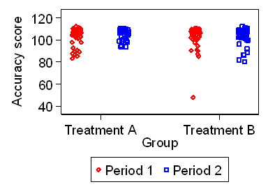
Figure 1 shows a plot of the accuracy score by treatment and period.

D

Figure 1. The accuracy test for the two periods and two treatments
(Observations have been jittered slightly so that they can be seen.)

The ceiling effect is apparent, and the distribution of the scores has a distribution which is negatively skew. It also appears that scores in Period 2 may be slightly greater than accuracy scores in Period 1.

We can do a simple test of the treatment effect, by estimating the mean difference, A minus B. I have used Stata for my analyses:

. ttest diffamb=0

One-sample t test

------------------------------------------------------------------------------
Variable |     Obs        Mean    Std. Err.   Std. Dev.   [95% Conf. Interval]
---------+--------------------------------------------------------------------
 diffamb |      84    1.035714      1.0045    9.206397   -.9621963    3.033625
------------------------------------------------------------------------------
Degrees of freedom: 83

                            Ho: mean(diffamb) = 0

     Ha: mean < 0               Ha: mean != 0              Ha: mean > 0
       t =   1.0311                t =   1.0311              t =   1.0311
   P < t =   0.8472          P > |t| =   0.3055          P > t =   0.1528

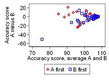
The estimated treatment effect = 1.0 (95% CI –1.0 to 3.0, P=0.3). However, we should ask whether the assumptions of this analysis are met by the data. The mean and standard deviation of the differences should be constant throughout the range, because we estimate them as single numbers. We can check this by a plot of the difference against average of the two scores, as in Figure 2.

D

Figure 2. Difference in accuracy scores against average of the two scores

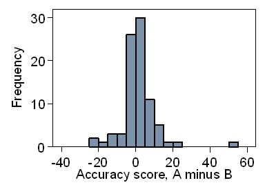
Clearly the standard deviation depends strongly on the accuracy. The differences should follow an approximately Normal distribution and the histogram (Figure 3) suggests that the tails are much too long.

D

Figure 3. Distribution of differences in accuracy scores

Hence we should try either a transformation or nonparametric test. I think that these data would be rather difficult to transform, because of the ceiling giving many zero differences at the top of the range. As the distribution of the differences is approximately symmetrical, we could use the Wilcoxon matched-pairs (signed rank) test.

The Stata output is:

. signrank diffamb=0

Wilcoxon signed-rank test

        sign |      obs   sum ranks    expected
-------------+---------------------------------
    positive |       36      1991.5      1739.5
    negative |       35      1487.5      1739.5
        zero |       13          91          91
-------------+---------------------------------
         all |       84        3570        3570

unadjusted variance    50277.50
adjustment for ties     -180.00
adjustment for zeros    -204.75
                     ----------
adjusted variance      49892.75

Ho: diffamb = 0
             z =   1.128
    Prob > |z| =   0.2592

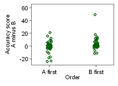
(A1 – B2) is the mean treatment difference for the group with A first, (A2 – B1) is the mean treatment difference for the group with A first. We can test the null hypothesis that the difference between these two mean differences is zero. We compare difference A minus B between orders. Figure 4 shows a scatter plot of the difference in accuracy score between treatments against treatment order.

D

Figure 4. Difference in accuracy score between treatments for the two treatment orders

We can compare the mean difference, A minus B, between the two orders using a two sample t test:

. ttest diffamb, by(order)  

Two-sample t test with equal variances

------------------------------------------------------------------------------
   Group |     Obs        Mean    Std. Err.   Std. Dev.   [95% Conf. Interval]
---------+--------------------------------------------------------------------
 A first |      43   -.8604651    1.295952    8.498127   -3.475803    1.754872
 B first |      41     3.02439    1.498978    9.598145   -.0051582    6.053939
---------+--------------------------------------------------------------------
combined |      84    1.035714      1.0045    9.206397   -.9621963    3.033625
---------+--------------------------------------------------------------------
    diff |           -3.884855    1.975746               -7.815243    .0455321
------------------------------------------------------------------------------
Degrees of freedom: 82

                Ho: mean(A first) - mean(B first) = diff = 0

     Ha: diff < 0               Ha: diff != 0              Ha: diff > 0
       t =  -1.9663                t =  -1.9663              t =  -1.9663
   P < t =   0.0263          P > |t| =   0.0527          P > t =   0.9737

The distribution in Figure 4 looks quite good for the t test, but we can compare the non-parametric analysis. This uses the Mann Whitney U test or two sample rank sum test:

. ranksum diffamb, by(order)  

Two-sample Wilcoxon rank-sum (Mann-Whitney) test

       order |      obs    rank sum    expected
-------------+---------------------------------
     A first |       43        1610      1827.5
     B first |       41        1960      1742.5
-------------+---------------------------------
    combined |       84        3570        3570

unadjusted variance    12487.92
adjustment for ties     -151.09
                     ----------
adjusted variance      12336.83

Ho: diffamb(order==A first) = diffamb(order==B first)
             z =  -1.958
    Prob > |z| =   0.0502

Again we have weak evidence of a period effect, P=0.05. The two analyses produce very similar results. So there appears to be some evidence for a learning effect in the accuracy score.

We can allow for a possible period effect by looking at the treatment difference for period 1, A1 – B1 and the treatment difference for period 2, A2 – B2, and averaging them to give (A1 – B1)/2 + (A2 – B2)/2. We can rearrange this:

      (A1 – B1)/2 + (A2 – B2)/2 = (A1 – B2)/2 – (B1 – A2)/2

Hence to estimate and test the treatment effect, we use the difference between the average difference between period 1, A1 – B2, and period 2, B1 – A2, for the two orders. This is called the CROS analysis. We get:

. ttest diff1m2, by(order)

Two-sample t test with equal variances
------------------------------------------------------------------------------
   Group |     Obs        Mean    Std. Err.   Std. Dev.   [95% Conf. Interval]
---------+--------------------------------------------------------------------
 A first |      43   -.8604651    1.295952    8.498127   -3.475803    1.754872
 B first |      41    -3.02439    1.498978    9.598145   -6.053939    .0051582
---------+--------------------------------------------------------------------
combined |      84   -1.916667    .9887793    9.062312   -3.883309    .0499756
---------+--------------------------------------------------------------------
    diff |            2.163925    1.975746               -1.766462    6.094313
------------------------------------------------------------------------------
    diff = mean(A first) - mean(B first)                          t =   1.0952
Ho: diff = 0                                     degrees of freedom =       82

    Ha: diff < 0                 Ha: diff != 0                 Ha: diff > 0
 Pr(T < t) = 0.8617         Pr(|T| > |t|) = 0.2766          Pr(T > t) = 0.1383

The estimate of the effect is half the observed difference: 2.163925/2 = 1.1 (95% CI –0.9 to 3.0, P=0.3). There is no evidence for a treatment effect.

The non-parametric equivalent is a Mann Whitney U test of the difference, period 1 minus period 2, between the two orders:

. ranksum diff1m2, by(order)

Two-sample Wilcoxon rank-sum (Mann-Whitney) test

       order |      obs    rank sum    expected
-------------+---------------------------------
     A first |       43        1949      1827.5
     B first |       41        1621      1742.5
-------------+---------------------------------
    combined |       84        3570        3570

unadjusted variance    12487.92
adjustment for ties     -100.77
                     ----------
adjusted variance      12387.15

Ho: diff1m2(order==A first) = diff1m2(order==B first)
             z =   1.092
    Prob > |z| =   0.2750

Again there is no evidence for a treatment effect, P=0.3. The two analyses give very similar results.

We can do the same analysis by analysis of variance, with accuracy score as the outcome variable and subject, treatment, and period as factors:

. anova score sub treat period

                           Number of obs =     170     R-squared     =  0.6490
                           Root MSE      = 6.40033     Adj R-squared =  0.2765

                  Source |  Partial SS    df       MS           F     Prob > F
              -----------+----------------------------------------------------
                   Model |  6210.08374    87  71.3802729       1.74     0.0059
                         |
                     sub |  5990.61699    85  70.4778469       1.72     0.0071
                   treat |  49.1391331     1  49.1391331       1.20     0.2766
                  period |  158.377228     1  158.377228       3.87     0.0527
                         |
                Residual |   3359.0692    82  40.9642585   
              -----------+----------------------------------------------------
                   Total |  9569.15294   169  56.6222068   

If we compare the results of the CROS analysis with the simple paired t test, we have treatment estimate 1.1 (95% CI –0.9 to 3.0, P=0.3) by CROS and estimated treatment effect = 1.0 (95% CI –1.0 to 3.0, P=0.3) by paired t test. In fact the P value for the CROS test is fractionally smaller, 0.28 compared to 0.31, and the confidence interval very slightly narrower, so ignoring the period effect has little impact on the results in this example.

In general though, it is better to take the period effect into account and do the CROS analysis. The period effect might be bigger than here and there is nothing to lose.

Back to top.

Interaction between period and treatment

We often want to ask whether the effects of B are the same if it follows A as they are if B comes first. In the mental fatigue trial, there could be an interaction because of the ceiling effect and practice improving accuracy. Treatment A could raise scores to the ceiling and all participants could get near the ceiling in the second period, due to practice. This would result in no treatment difference if A came first, but a difference if B came first.

We ask whether the treatment difference is the same whatever order of treatments is given. In other words, is there an interaction between period and treatment? Is there an order effect? If there is no interaction, the participant’s average response should be the same whichever order treatments were given. We ask: is A1 + B2 = A2 + B1? Note that this is the same as comparing the treatment difference in period 1 with the treatment difference in period 2:

      is A1 – B1 = A2 – B2?

To test for a period × treatment interaction, we can compare the sum or the average of the scores on the two treatments between orders. The participant’s average response should be the same in whichever order treatments are given.

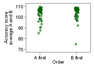
Figure 5 shows the average score for treatments A and B plotted against the order in which treatments were given.

D

Figure 5. Average score for treatments A and B by order in which treatments were given

We can compare average between orders using a two sample t test:

. ttest av1and2, by(order)  

Two-sample t test with equal variances

------------------------------------------------------------------------------
   Group |     Obs        Mean    Std. Err.   Std. Dev.   [95% Conf. Interval]
---------+--------------------------------------------------------------------
 A first |      43     102.593    .9138191    5.992312    100.7489    104.4372
 B first |      41    103.2439    .9346191    5.984482     101.355    105.1328
---------+--------------------------------------------------------------------
combined |      84    102.9107    .6504313    5.961301     101.617    104.2044
---------+--------------------------------------------------------------------
    diff |           -.6508792    1.307167               -3.251251    1.949493
------------------------------------------------------------------------------
Degrees of freedom: 82

                Ho: mean(A first) - mean(B first) = diff = 0

     Ha: diff < 0               Ha: diff != 0              Ha: diff > 0
       t =  -0.4979                t =  -0.4979              t =  -0.4979
   P < t =   0.3099          P > |t| =   0.6199          P > t =   0.6901

There is no evidence of an interaction, P=0.6. However, the distributions shown in Figure 5 are negatively skew, not Normal and the assumptions for the t test are not well met.

We can do a Mann Whitney U test instead:

. ranksum av1and2, by(order)  

Two-sample Wilcoxon rank-sum (Mann-Whitney) test

       order |      obs    rank sum    expected
-------------+---------------------------------
     A first |       43        1766      1827.5
     B first |       41        1804      1742.5
-------------+---------------------------------
    combined |       84        3570        3570

unadjusted variance    12487.92
adjustment for ties      -67.77
                     ----------
adjusted variance      12420.15

Ho: av1and2(order==A first) = av1and2(order==B first)
             z =  -0.552
    Prob > |z| =   0.5811

Again we have P = 0.6 and no evidence of any interaction between treatment and order in this trial.

The power of the test of interaction is low and alpha = 0.10 is often recommended as a decision point, rather that 0.05. As we shall see below, the real question is whether we should test at all and what we should do if we find anything.

Back to top.

Carry over effects

In the mental fatigue trial, there could be an interaction because of the ceiling effect and practice. Another possibility in cross-over trials is a carry-over effect, where the first treatment continues to have an effect in the second period.

This example, a trial of Nicardipine against placebo in patients with Raynaud’s phenomenon (Kahan et al., 1987) was given by Altman (1991). Patients with Raynaud’s phenomenon were given either the drug Nicardipine or a placebo, each for a two week period, in random order. They were asked to record the number of attacks of Raynaud’s phenomenon which they experienced. Table 3 shows the results.

Table 3. Attacks of Raynaud’s phenomenon in two week periods

Nicardipine first			Placebo first
Period 1 Nicardipine	Period 2 Placebo	Placebo – Nicardipine	Period 1 Placebo	Period 2 Nicardipine	Placebo – Nicardipine
16	12	– 4	18	12	6
26	19	–7	12	4	8
8	20	12	46	37	9
37	44	7	51	58	–7
9	25	16	28	2	26
41	36	–5	29	18	11
52	36	–16	51	44	7
10	11	1	46	14	32
11	20	9	18	30	–12
30	27	–3	44	4	40
Means:
24.0	25.0	1.0	34.3	22.3	12.0

When Nicardipine was the first treatment, there was no obvious difference between Nicardipine and placebo and the mean difference was only 1.0 attacks. When placebo was the first treatment, there was a much larger difference between Nicardipine and placebo and the mean difference was 12.0 attacks. That looks like carry-over to me! The Nicardipine appears to be still acting when the subject takes the placebo. 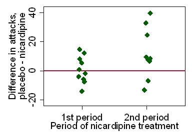Figure 6 shows the difference in numbers of attacks on placebo and on Nicardipine for the two treatment orders.

D

Figure 6. Difference in attacks of Raynaud’s phenomenon on Nicardipine and placebo by treatment order, with zero line

There is a line through zero, clearly showing that the differences are scattered equally about zero for Nicardipine first and mostly above zero for placebo first.

We can test for an interaction between treatment and period by comparing the average of the two periods between the two orders:

. ttest av , by(order)

Two-sample t test with equal variances
------------------------------------------------------------------------------
   Group |     Obs        Mean    Std. Err.   Std. Dev.   [95% Conf. Interval]
---------+--------------------------------------------------------------------
1st peri |      10        24.5    3.952496    12.49889    15.55883    33.44117
2nd peri |      10        28.3    4.782027     15.1221     17.4823     39.1177
---------+--------------------------------------------------------------------
combined |      20        26.4    3.050582    13.64262    20.01506    32.78494
---------+--------------------------------------------------------------------
    diff |                -3.8    6.204031               -16.83419    9.234185
------------------------------------------------------------------------------
    diff = mean(1st peri) - mean(2nd peri)                        t =  -0.6125
Ho: diff = 0                                     degrees of freedom =       18

    Ha: diff < 0                 Ha: diff != 0                 Ha: diff > 0
 Pr(T < t) = 0.2739         Pr(|T| > |t|) = 0.5479          Pr(T > t) = 0.7261

. ttest diff1m2, by(order)

Two-sample t test with equal variances
------------------------------------------------------------------------------
   Group |     Obs        Mean    Std. Err.   Std. Dev.   [95% Conf. Interval]
---------+--------------------------------------------------------------------
1st peri |      10          -1    3.119829    9.865766   -8.057544    6.057544
2nd peri |      10          12    5.168279    16.34353    .3085399    23.69146
---------+--------------------------------------------------------------------
combined |      20         5.5    3.294733    14.73449   -1.395955    12.39595
---------+--------------------------------------------------------------------
    diff |                 -13    6.036923               -25.68311   -.3168945
------------------------------------------------------------------------------
    diff = mean(1st peri) - mean(2nd peri)                        t =  -2.1534
Ho: diff = 0                                     degrees of freedom =       18

    Ha: diff < 0                 Ha: diff != 0                 Ha: diff > 0
 Pr(T < t) = 0.0225         Pr(|T| > |t|) = 0.0451          Pr(T > t) = 0.9775
Evidence for a treatment effect, P = 0.045.  

. ttest diffamb=0

One-sample t test
------------------------------------------------------------------------------
Variable |     Obs        Mean    Std. Err.   Std. Dev.   [95% Conf. Interval]
---------+--------------------------------------------------------------------
 diffamb |      20         6.5     3.19745    14.29943    -.192339    13.19234
------------------------------------------------------------------------------
    mean = mean(diffamb)                                          t =   2.0329
Ho: mean = 0                                     degrees of freedom =       19

    Ha: mean < 0                 Ha: mean != 0                 Ha: mean > 0
 Pr(T < t) = 0.9719         Pr(|T| > |t|) = 0.0563          Pr(T > t) = 0.0281

Back to top.

Should we test the period × treatment interaction?

Should we test for an interaction in a crossover trial? And what should we do about it when there is one? There are two views about this. One follows Grizzle (1965). He recommended testing the interaction routinely. He argued that if the interaction were significant, we cannot use the tainted second period. We should use the period 1 data only.

If we do this for the fatigue trial, we get difference, A – B = 0.5 (95% CI –3.2 to 4.2, P=0.8). This approach is called the two-stage analysis. Its proponents recommend that we should do the cross-over trial with a sufficient sample size to have adequate power from a two-group comparison of period 1 only. This seems to contradict the whole purpose of a cross-over trial, sacrificing its greater efficiency.

If we compare the full data estimate using the CROS analysis, our estimated difference, A – B, = 1.1 (95% CI –0.9 to 3.0, P=0.3). The confidence interval is narrower and the P value smaller. With the two stage analysis we lose power and precision.

For the Nicardipine data, the estimate for the first period only is given by:

. ttest per1, by( order)

Two-sample t test with equal variances
------------------------------------------------------------------------------
   Group |     Obs        Mean    Std. Err.   Std. Dev.   [95% Conf. Interval]
---------+--------------------------------------------------------------------
1st peri |      10          24    4.935135    15.60627    12.83595    35.16405
2nd peri |      10        34.3    4.740019    14.98926    23.57733    45.02267
---------+--------------------------------------------------------------------
combined |      20       29.15    3.533505    15.80231    21.75429    36.54571
---------+--------------------------------------------------------------------
    diff |               -10.3    6.842758                -24.6761    4.076101
------------------------------------------------------------------------------
    diff = mean(1st peri) - mean(2nd peri)                        t =  -1.5052
Ho: diff = 0                                     degrees of freedom =       18

    Ha: diff < 0                 Ha: diff != 0                 Ha: diff > 0
 Pr(T < t) = 0.0748         Pr(|T| > |t|) = 0.1496          Pr(T > t) = 0.9252

This is not significant, P = 0.15, compared to P = 0.045 by CROS.

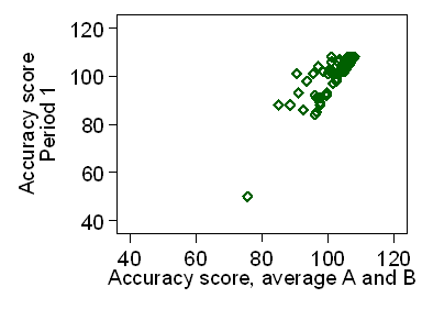
Senn (1989) argued that the interaction test is highly misleading. The average of the first and second periods is highly correlated with the first period. For the fatigue trial, this is shown in Figure 7, where the accuracy score in the first period can be seen to be quite strongly related to the average of the two.

D

Figure 7. Accuracy score for Period 1 against the average accuracy score over both periods

Hence the treatment test using first period only is highly correlated with the interaction test. The alpha value for the first period test conditional on the interaction test is much greater than 0.05.

I find this argument entirely persuasive. In any case, if the interaction is significant, there is a significant treatment effect. An interaction means that the treatment effect is different for different orders and for this to be true there must be a treatment effect in the first place.

In their text book, Jones and Kenward (1989) review the question but do not make a strong recommendation. I find Senn’s argument convincing. I would say do not test or do the two-stage analysis.

However, I think it is worth inspecting the data to see whether the assumption of no interaction required for the CROS estimate is plausible. If it is not, rely on the P value. Hence in the Nicardipine trial, the assumption of no interaction is not plausible, even though the test for it is not significant. I think the CROS estimate would be an underestimate. Despite this, I think that the significance test does reflect there being sufficient evidence for us to conclude that Nicardipine has an effect.

If we suspect carry-over, whether we test for it not, what should we do instead of Grizzle’s approach using the first period only? Senn (1989) suggested that if the estimate is needed, rather than evidence of the existence of an effect, we should repeat the trial and design the carry-over out of it, using washout periods as described next.

Back to top.

Washout periods

A washout period is a time when the participants do not receive any active trial treatment. It is intended to prevent continuation of the effects of the trial treatment from one period to another, carry-over. A typical cross-over trial with washout periods might look like this:

1. Washout / run-in — removes effects of pre-trial treatments
2. Treatment 1
3. Washout — removes effects of treatment 1
4. Treatment 2
5. Washout — removes effects of treatment 2
6. Usual care

A washout period is necessary if treatments might interact in an adverse way. If two drugs are being compared which have antagonistic methods of action, we do not them both to be present at the same time.

In a placebo controlled trial, we do not need washout periods for safety reasons. We could simply make the treatment periods long enough so that the first treatment has been eliminated by the time we make the measurements for the second treatment.

In drug trials, washout periods should be at least 3 × half life of drug in body (FDA). If no washout periods are used, the treatment periods should be longer than would be required for washout and no measurements made in the time that would be needed for washout.

Back to top.

Baseline measurements

Baseline measurements are made before we begin the trial. In a cross-over trial, baseline measurements may be made before the trial treatments begin:

1. Washout
2. Baseline 1
3. Period 1 outcome
4. Period 2 outcome

or at the start of each period:

1. Washout
2. Baseline 1
3. Period 1 outcome
4. Washout
5. Baseline 2
6. Period 2 outcome

In a parallel group trial, baseline measurements can be very useful as covariates and can greatly improve power or reduce required sample size. They are of less value in cross-over trials.

As in a parallel group trial, Baseline 1 can be used as a descriptive variable for the trial population, so that we know what kind of participants are taking part in the trial. We can also use Baseline 1 to look for a baseline × treatment interaction, e.g. do people with high baseline values of the outcome measurement have a different treatment effect from people with low baseline values? This requires a larger sample than required to detect the overall treatment effect to be worthwhile.

With only one baseline, we can also include it as a treatment period, to give a three period design and use it to improve the estimate of variance. This might be of some limited value in very small trials where we have few degrees of freedom.

When there are two baselines, we can include them as covariates in an analysis of covariance. This may increase power and improve the estimate. We make the treatment period the unit of analysis and use subject, treatment, and period or treatment order as categorical factors and baseline for the period as a continuous covariate. This might be of value if the level of the outcome would be changing slowly over time in the absence of a trial, but it runs the risk of being distorted because the effects of the first treatment are still present at the time of the second baseline. We must have an adequate washout period to do this. Just as in a parallel group trial, we should not use differences from baseline as our outcome variable. This increases the measurement error. Comparing two differences from baseline in a cross-over trial would give four lots of measurement error rather than two and we would lose power.

Although we can make some use of them, baseline measurements are not really necessary in a cross-over trial. The comparison is within the trial participant anyway.

Back to top.

Books on cross-over trials

There are two text-books devoted to cross-over trials. I have referred to both, but they both now have second editions, Senn (2002) and Jones and Kenward (2003). For a brief introduction, try Altman (1991).

Back to top.

References

Altman DG. (1991) Practical Statistics for Medical Research. Chapman and Hall, London.

Grizzle JE. (1965) The two-period change-over design and its use in clinical trials. Biometrics, 21: 467-480.

Jones B and Kenward MG. (1989) Design and Analysis of Cross-Over Trials. London: Chapman and Hall.

Jones B and Kenward MG. (2003) Design and Analysis of Cross-Over Trials, 2nd ed. London: Chapman and Hall.

Kahan A, Amor B, Menkes CJ, et al. (1987) Nicardipine in the treatment of Raynaud’s phenomenon: a randomised doubleblind trial. Angiology 38: 333-7.

Pritchard BNC, Dickinson CJ, Alleyne GAO, Hurst P, Hill ID, Rosenheim ML, Laurence DR. (1963) Report of a clinical trial from Medical Unit and MRC Statistical Unit, University College Hospital Medical School, London. British Medical Journal 2: 1226-7.

Senn S. (1989) Cross-Over Trials in Clinical Research. Chichester: Wiley.

Senn S. (2002) Cross-Over Trials in Clinical Research, 2nd ed. Chichester: Wiley.

Back to top.

To Trials course index.

To Martin Bland's M.Sc. index.

To Martin Bland's home page.

This page maintained by Martin Bland.
Last updated: 15 September, 2010.

Back to top.