Sample size for clinical trials

• Outcome variables for trials
• How large a sample should I take?
• Comparison of two means
• More practical methods of calculation
• Other sample size considerations
• Comparing two proportions
• Expressing differences between two proportions
• Other factors affecting power
• References

Outcome variables for trials

An outcome variable is one which we hope to change, predict or estimate in a trial.

Examples:

• Systolic blood pressure in a hypertension trial
• Caesarean section rate in an obstetric trial
• Survival time in a cancer trial

How many outcome variables should I have? If we have many outcome variables:

• all possibilities would be covered,
• we would be less likely to miss something,
• the risk of false positives, finding an apparent effect when there is none in reality, would be increased.

If we have few outcome variables:

• the trial would be easier and quicker to check and analyse,
• the trial would be cheaper,
• the trial would be easier for research subjects,
• we would avoid multiple testing and the high risk of a false positive result,
• we might miss something important.

We get round the problem of multiple testing by having one outcome variable on which the main conclusion stands or falls, the primary outcome variable. If we do not find an effect for this variable, the study has a negative result. Usually we have several secondary outcome variables, to answer secondary questions. A significant difference for one of these would generate further questions to investigate rather than provide clear evidence for a treatment effect. The primary outcome variable must relate to the main aim of the study. Choose one and stick to it.

Back to top.

How large a sample should I take?

A significance test for comparing two means is more likely to detect a large difference between two populations than a small one. The probability that a test will produce a significant difference at a given significance level is called the power of the test. The power of a test is related to:

• the postulated difference in the population,
• the standard error of the sample difference (which depends on the sample size)
• the significance level, usually 0.05, chosen in advance. .

The relationship between:

• power of the test, P
• postulated difference in the population, δ
• standard error of the sample difference, SE(d)
• significance level, α

If we know three of these we can calculate the fourth.

ƒ(α,P) depends on power and significance level only.

Values of ƒ(α,P) for different P and α:

P	α
	0.05	0.01
0.50	3.8	6.6
0.70	6.2	9.6
0.80	7.9	11.7
0.90	10.5	14.9
0.95	15.2	20.4
0.99	18.4	24.0

Usually we choose the significant level to be 0.05 and P to be 0.80 or 0.90, so the numbers we actually use from this table are 7.9 and 10.5.

We can then choose the difference we want the trial to detect, δ, and from this work out what sample size we need.

For an example, consider a trial of treatments intended to reduce blood pressure. We want to compare two treatments. We decide that a clinically important difference would be 10 mm Hg. Where does this difference come from? It could be

• Clinical judgement as to what would be important. This might come from a focus group of clinicians or patients, for example.
• What the treatment might achieve. This might come from pilot studies, or other trials of similar treatments.
• Back calculation from what is feasible. We start with the sample size we think we can get, then work from there back to the difference this sample size could detect. This is rightly frowned on by referees.

Having chosen the difference we want our trial to be able to detect if it exists, δ, we can then use this and the chosen power, P, and significance level, α, calculate the required standard error of the sample difference, SE(d). SE(d) depends on the required sample size, n, and the variability of the observations. How SE(d) depends these things depends in turn on the particular sample size problem.

Back to top.

Comparison of two means

Compare the means of two samples, sample sizes n₁ and n₂, from populations with means μ₁ and μ₂, with the variance of the measurements being σ².

We have d = μ₁ – μ₂ and

so the equation becomes:

For equal sized groups, n₁ = n₂ = n, the equation becomes:

Consider the example of a trial of an intervention for depression in primary care The primary outcome will be the PHQ9 depression score after 4 months. The PHQ9 scale is from 0 to 27, a high score = depressed. We decide a clinically important difference would be 2 points on the PHQ9 scale. From a pilot study, we find that the standard deviation of PHQ9 after treatment = 7 scale points. We shall choose power P = 0.90 = 90%, α = 0.05 =5%. Hence ƒ(α,P) = 10.5.

We want to detect difference δ = μ₁ – μ₂ = 2.

becomes

which gives

Hence we need 258 patients in each group.

Back to top.

More practical methods of calculation

That’s the hard way to do it. We can also use:

• Software, e.g. nQuery Advisor
• Graphics, e.g. Altman’s nomogram
• Tables, e.g. Machin, et al. (1998) Statistical Tables for the Design of Clinical Studies, Second Edition.

Software

PS can be downloaded from www.mc.vanderbilt.edu/prevmed/ps/.

If you download and start PS, you can click continue to get into the program proper. To compare two means, click “t test”. For “What do you want to know" click “Sample size”. For “Paired or independent” click “Independent”. Now put in alpha = 0.05, power = 0.90, delta = 2, and sigma = 7. The rather mysterious “m” is the number of subjects in the second group for each subject in the first group, it enables you to have unequal group sizes. Put in “1”. Now click “Calculate” and you should see the sample size per group, 258.

For smaller samples, PS may get a larger sample size than my formula. This is because it allows for the degrees of freedom in a t test. My formula is for a large sample Normal test and so does not allow for this. The smaller the indicated sample is, the further apart the formula and PS will be. PS is better.

Not too hard, is it, really? You can also put in the difference and sample size and calculate the power, or the sample size and power and calculate the difference you could detect. This is the method I usually use for sample size calculations.

Altman’s nomogram

Altman’s nomogram is a very clever graphical method for calculating sample sizes, devised by my long-time collaborator Doug Altman. You can find a copy of Altman’s nomogram in his excellent book Practical Statistics for Medical Research or on many sites on the World Wide Web, e.g. http://www.pubmedcentral.nih.gov/articlerender.fcgi?artid=137461. Download a copy and print it out if you want to try it.

To use the nomogram, we first need to translate our required difference into the effect size or standardized difference. This is the difference in measured in standard deviations. We find our difference divided by the standard deviation.

For the depression example, the required difference = 2 and the standard deviation = 7 mm Hg. The effect size = 2/7 = 0.286. If our measurement have units, these cancel out, this is a pure number and would be the same whatever units we used to measure depression.

Here is the nomogram, a graphical tool for calculation:

D

Now, mark the standardised difference on the left vertical scale and the power on the right vertical scale. We draw a line between these points:

D

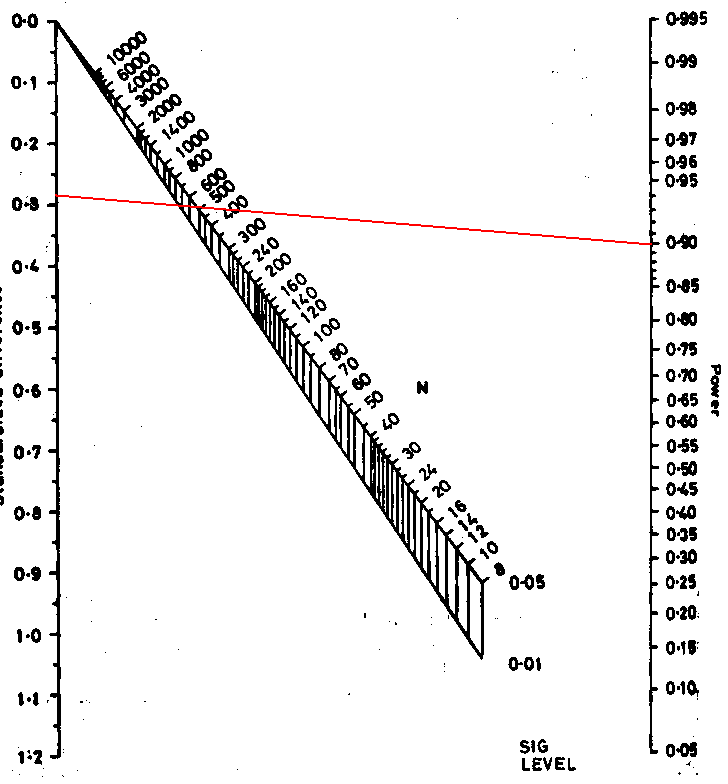
Where this line intersects the middle sloping lines gives the sample size for significance levels 0.05 and 0.01. Reading off the scale we get N = 520. This the total sample size required, and so gives 520/2 = 260 in each group, as before, apart from the inaccuracy caused by reading the scale. This nomogram embodies the large sample formula, not the better t test method used by PS.

Tables

The book by Machin et al., Statistical Tables for the Design of Clinical Studies, Second Edition. gives many tables for sample size calculation. It also discusses many sample size problems.

Back to top.

Other sample size considerations:

The decisions about difference to be detected and power, then the actual calculations, are not the only problems with sample size. Having estimated it, we might then find that

• Eligible patients disappear like snow in August. Clinicians are often very optimistic about how many suitable patients they see.
• Eligible patients may refuse.
• Clinicians may forget or refuse to enrol eligible patients.
• Patients may drop out.

We often allow for this by increasing the sample size. Inflations between 10% and 20% are popular. We should also make sure that the new sample size is much smaller than the predicted number of eligible patients. Getting patients into clinical trials is NOT easy.

Back to top.

Comparing two proportions:

This is the most frequent sample size calculation. We have two proportions p₁ and p₂. Unlike the comparison of means, there is no standard deviation. SE(d) depends on p₁ and p₂ themselves.

The equation becomes

There are several different variations on this formula. Different books, tables, or software may give slightly different results. If we have two equal groups, it becomes:

For an example, consider a trial of an intervention to reduce the proportion of births by Caesarean section. We will take the usual power and sample size P = 0.90, α = 0.05, so ƒ(α,P) = 10.5.

From clinical records we observe 24% of births are by Caesarean section and decide that a reduction to 20% would be of clinical interest. We have p₁ = 0.24, p₂ = 0.20. The calculation proceeds as follows:

So n = 2,247 in each group.

Detecting small differences between proportions requires a very large sample size.

We can do the same calculation using PS. We choose “dichotomous”, because our outcome variable, Caesarean section, is yes or no. We then proceed as for the comparison of two means. For “What do you want to know click “Sample size”, for “Paired or independent” click “Independent”. We now have a new question, “Case control?”, to which we answer “Prospective”, because a clinical trial is a prospective study. The alternative hypothesis is expressed as two proportions. To correspond to the large sample formula above, the testing method would be uncorrected chi-squared. You could choose “Fisher’s exact test” if you were feeling cautious. There is a lot of statistical argument about this choice and we will not go into it here. Now put in α = 0.05, power = 0.90, p₁ = 0.24, p₂ = 0.20, and m = 1. Click “Calculate” and you should see the sample size per group, 2253. Not quite the same as my formula gives, but very similar.

You can also use the nomogram for this calculation.

Back to top.

Expressing differences between two proportions

As percentages, the proportions are p₁ = 24%, p₂ = 20%, so the difference = 4. Are we looking for a reduction of 4% in Caesarean sections? No we are not! A reduction of 4% would be 4% of 24% = 4–24/100 = 0.96, i.e. from 24% down to 23.04%. The reduction from 24% to 20% is 4 percentage points, NOT 4%.

This is important, as I see trials described as aiming to detect a reduction of 20% in mortality, when this is from 30% down to 10%. That is a reduction of 20 percentage points, or 67%.

Back to top.

Other factors affecting power

Power may be increased by

• adjustment for baseline and prognostic variables.

Power may be reduced by

• cluster randomisation.

If in doubt, consult a statistician.

Back to top.

Allowing for adjustment

Power may be increased by adjustment for baseline and prognostic variables. We need to know the reduction in the standard deviation produced by the adjustment. Researchers often simply say: “Power will be increased by adjustment for . . .”. so that things will actually be be better than they estimate, but they cannot say by how much.

When we do regression, the regression removes some of the variability, in that the variance of of the residuals, the observed values of the outcome variable minus the values predicted by the regression equation, is less than the variance of the outcome variable before regression. The proportion of variation explained by regression = r², where r is the correlation coefficient, and the variance after regression is equal to the variance before regression multiplied by (1 − r²). Hence the standard deviation after regression is σ√(1 − r²).

For example, suppose we want to do a trial of a therapy programme for the management of depression. We measure depression using the PHQ9 scale, which runs from 0 to 27, and a high score = depression. We want to design a trial to detect a difference in mean PHQ9 = 2 points. From an existing trial, we know that people identified with depression in primary care and given treatment as usual have baseline PHQ9 score with mean = 18 and SD = 5. After four months they had mean = 13, SD = 7, correlation r = 0.42.

We will do a power calculation, choosing power = 0.90, significance level = 0.05, difference = 2, and SD = 7. This gives sample size n = 258 per group. We also know r = 0.42. The standard deviation after regression will be σ√(1 − r²). = 7×√(1 − 0.42²) = 6.35. We now repeat the power calculation with power = 0.90, significance level = 0.05, difference = 2, and SD = 6.35. This gives n = 213 per group.

If we have a good idea of the reduction in the variability that regression will produce, we can use this to reduce the required sample size. The effect is not usually very great. For example, to halve the required sample size, we must have (1 − 0.42²) = 1/2, so r² = 1/2, so r = 0.71. 0.71 is a pretty big correlation coefficient.

Confidence intervals

There has been a movement to present the results of trials in the form of confidence intervals rather than P values (Gardner and Altman 1986). This was motivated by the difficulties of interpreting significance tests, particularly when the result was not significant. This campaign was very successful and many major medical journals changed their instructions to authors to say that confidence intervals would be the preferred or even required method of presentation. This was later endorsed by the wide acceptance of the CONSORT standard for the presentation of clinical trials. We insist on interval estimates and rightly so.

If we ask researchers to design studies the results of which will be presented as confidence intervals, rather than significance tests, I think that we should base our sample size calculations on confidence intervals, rather than significance tests. It is inconsistent to say that we insist on the analysis using confidence intervals but the sample size should be decided using significance tests (Bland 2009).

How do we do this? We need a formula for the confidence interval for the treatment difference in terms of the expected parameters and sample size. We must decide how precisely we want to estimate the treatment difference.

For a large study, the 95% confidence interval will be 1.96 standard errors on either side of the observed difference. For a trial with equal sized samples, the 95% confidence interval for the difference between two means will be ±1.96σ√(2/n) and for two proportions it will be ±1.96√(p₁(1 − p₁)/n + p₂(1 − p₂)/n)

For example, the International Carotid Stenting Study (ICSS) was designed to compare angioplasty and stenting with surgical vein transplantation for stenosis of carotid arteries, to reduce the risk of stroke. We did not anticipate that angioplasty would be superior to surgery in risk reduction, but that it would be similar in effect. The primary outcome variable was to be death or disabling ipsilateral stroke after three years follow-up. There was to be an additional safety outcome of death, stroke, or myocardial infarction within 30 days and a comparison of cost. The sample size calculations for ICSS were based on the earlier CAVATAS study, which had the 3 year rate for ipsilateral stroke lasting more than 7 days = 14%. The one year rate was 11%, so most events were within the first year. There was very little difference between the treatment arms.

This was an equivalence trial, no difference was anticipated, p₁ = p₂ = 0.14. The width of the confidence interval for the difference between two very similar percentages is given by ±1.96√(p₁(1 − p₁)/n + p₂(1 − p₂)/n) If we put p₁ = p₂ = 0.14, we can calculate this for different sample sizes:

Sample size	Width of 95% confidence interval
250	±0.061
500	±0.043
750	±0.035
1000	±0.030

We chose 750 in each group.

For two means, width of the 95% confidence interval for the difference = ±1.96σ√(2/n). If we put n = 740, we can calculate this for the chosen sample size: ±1.96σ√(2/750) = ±0.10σ. This was thought to be ample for cost data and any other continuous variables.

References

Altman, D.G. (1991) Practical Statistics for Medical Research. Chapman and Hall, London.

Bland M. (2000) An Introduction to Medical Statistics. Oxford University Press.

Bland JM. (2009) The tyranny of power: is there a better way to calculate sample size? British Medical Journal 339: b3985.

CAVATAS investigators. (2001) Endovascular versus surgical treatment in patients with carotid stenosis in the Carotid and Vertebral Artery Transluminal Angioplasty study (CAVATAS): a randomised trial. Lancet 357: 1729-37.

Featherstone RL, Brown MM, Coward LJ. (2004) International Carotid Stenting Study: Protocol for a randomised clinical trial comparing carotid stenting with endarterectomy in symptomatic carotid artery stenosis. Cerebrovascular Disease 18: 69-74.

Gardner MJ and Altman DG. (1986) Confidence intervals rather than P values: estimation rather than hypothesis testing. British Medical Journal 292: 746-50.

Machin, D., Campbell, M.J., Fayers, P., Pinol, A. (1998) Statistical Tables for the Design of Clinical Studies, Second Edition. Blackwell, Oxford.

nQuery Advisor, http://www.statistical-solutions-software.com/ (commercial software)

PS Power and Sample Size, http://biostat.mc.vanderbilt.edu/wiki/Main/PowerSampleSize (free Windows program)

Back to top.

To Trials course index.

To Martin Bland's M.Sc. index.

To Martin Bland's home page.

This page maintained by Martin Bland.
Last updated: 26 October, 2011.

Back to top.