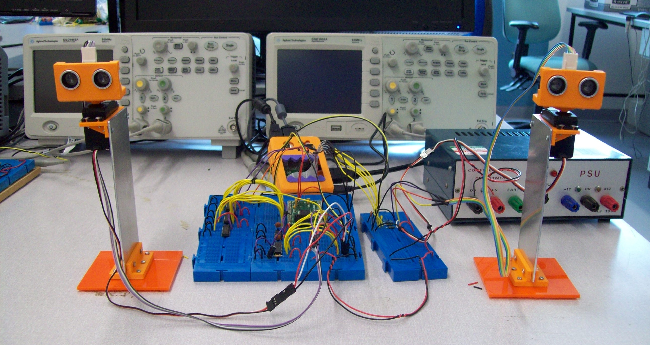
Figure 1 : System
This project was designed to show that you can't solve every problem in software, that you need to understand a system's limitations and that adding hardware can actually simplify software development. Aim: to implement a system that scans 180 degrees, measure the distance to the nearest obstacle and display these as a polar plot. One system will be implemented in software (as much as possible), another using both software and dedicated hardware. Both systems use a common sensor platform as shown in figure 2. Position control is implemented using a standard analogue model servo (Link), distance measurement via an off the shelf, HC-SR04 ultrasonic module (Link). The 3D printed brackets where obtained from: (Link) (Link), the bottom base bracket was quickly done in openScad (Link). The base was laser cut, layout drawn in LibreCad (Link). All 3D model and dxf files are available here (Local).
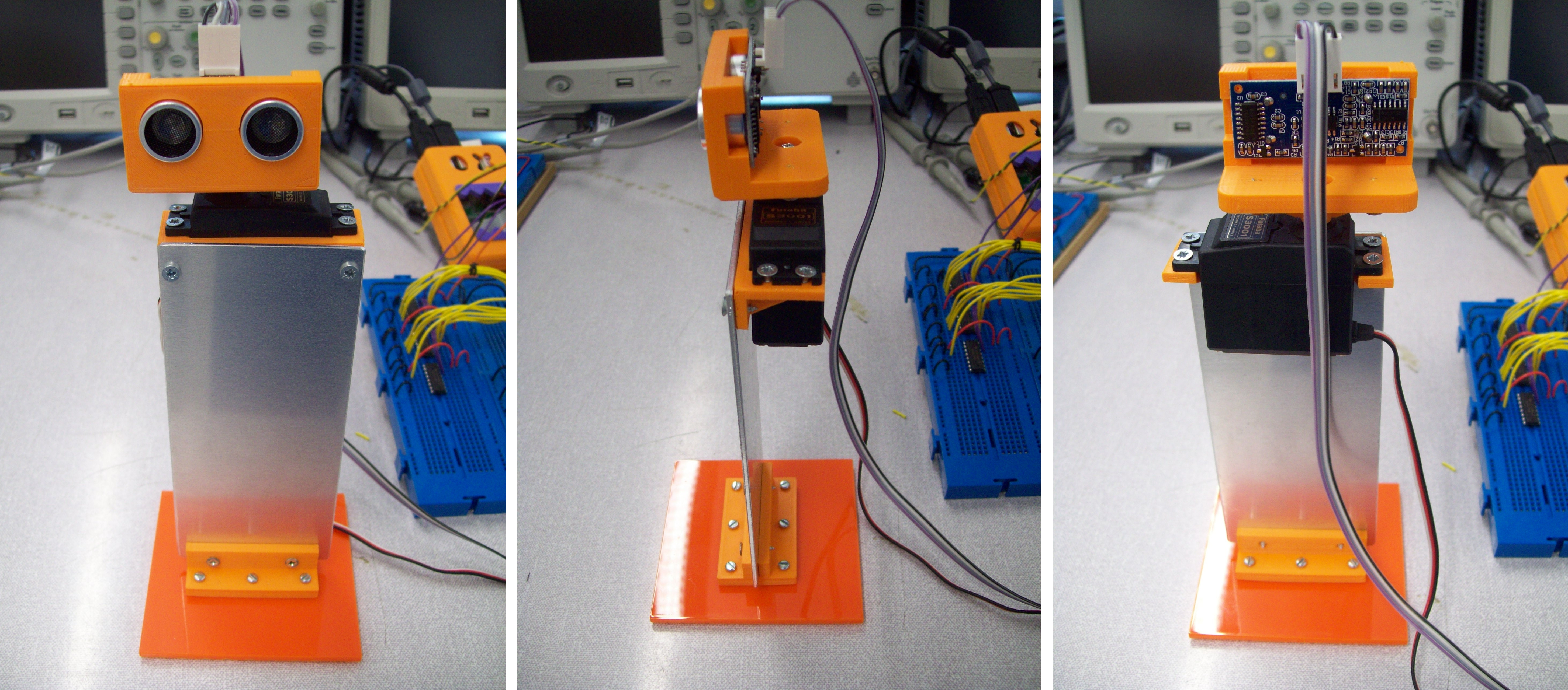
Figure 2 : Sensor platform
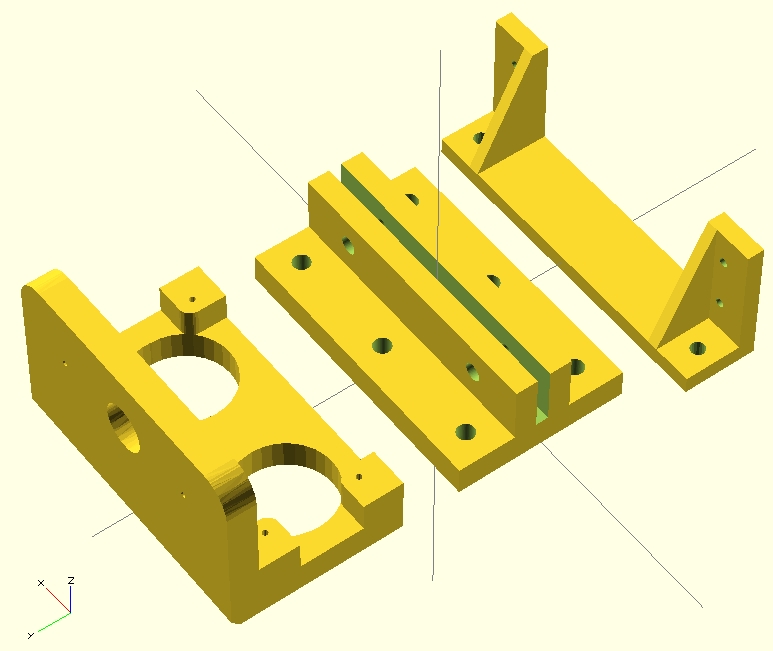
Figure 3 : 3D printed parts
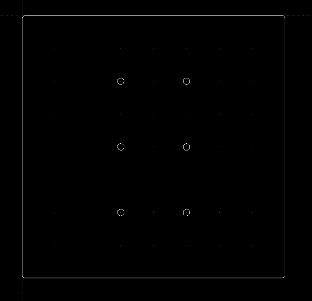
Figure 4 : Plastic base
The software biased system requires minimal external hardware, as shown in figures 5 and 6. The resistors shown are purely for protection i.e. the Raspberry Pi is not 5V tolerant. Resistors R2 and R4 are not really needed, these are 41 ohms (were to hand), just there to limit the current if i do something silly. Resistors R1 and R3 (4K7) form a potential, shifting the ultrasonic module's output pulse from 5V down to 2.5V i.e. Pi safe.
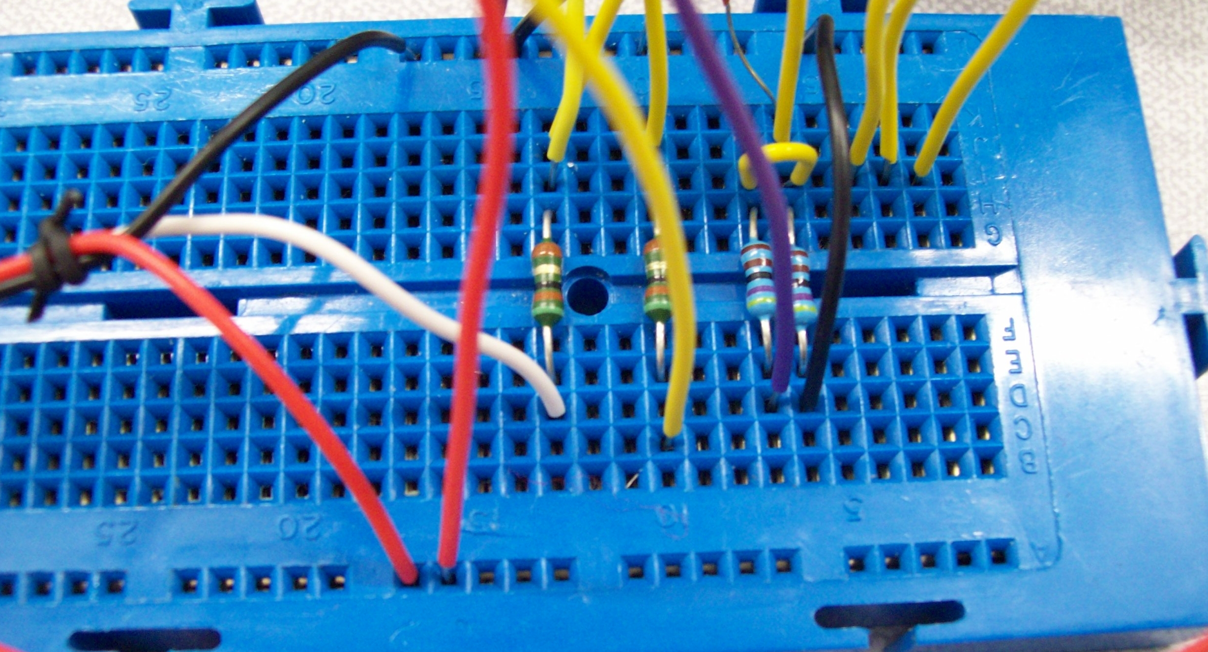
Figure 5 : Software system interface
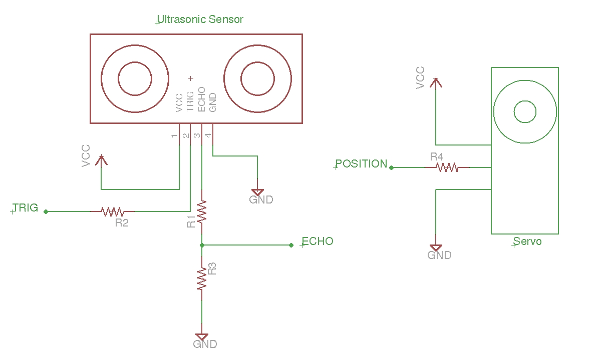
Figure 6 : Software interface circuit diagram
The servo and ultrasonic sensor are controlled using a simple python prgram. The ultrasonic sensor control was based on this example: (Link) (Local). The servo control was based on this example: (Link) (Local). The full code listing is shown below:
import RPi.GPIO as GPIO
import time

# Servo position control func
def update(angle):
	duty = float(angle) / 10 + 2.5
	pwm.ChangeDutyCycle(duty)

#IO pin numbers
TRIG = 17
ECHO = 27
SERVO = 18

#Setup IO ports
GPIO.setwarnings(False)
GPIO.setmode(GPIO.BCM)

GPIO.setup(TRIG, GPIO.OUT)
GPIO.setup(ECHO, GPIO.IN)

GPIO.setup(SERVO, GPIO.OUT)

pwm = GPIO.PWM(SERVO, 100)
pwm.start(5)

GPIO.output(TRIG, False)

#Initialise variables
direction = True
angle = 0
pos = 0
pos_prev = 17
pulse_start = 0
pulse_end = 0

b = [ 0,0,0,0,0,0,0,0,0,0,0,0,0,0,0,0,0,0,0 ]
c = [ 0,0,0,0,0,0,0,0,0,0,0,0,0,0,0,0,0,0,0 ]

#Main loop
while True :
	#Send trigger (start) pulse to US sensor
	GPIO.output(TRIG, True)
	time.sleep(0.00001)
	GPIO.output(TRIG, False)

	#Wait until RX signal 0 or max delay
	timeout = 0
	while (GPIO.input(ECHO)==0) and (timeout < 50):
		timeout = timeout + 1
		pulse_start = time.time()

	#Wait for RX signal
	while GPIO.input(ECHO)==1:
		pulse_end = time.time()

	#Calculate time of flight
	pulse_duration = pulse_end - pulse_start

	#convert time to distance
	distance = pulse_duration * 17150
	distance = round(distance, 2)

	#Trap if no pulse recieved
	if distance < 0:
		distance = 0

	distance = distance * 10

	#Set max distance for display
	if distance > 600:
		distance = 600

	print "Distance: ", distance,"mm", "Angle: ", pos

	#Move sensor head
	update(angle)
	time.sleep(0.5)

	#update log file
	file = open('plot_1.dat', 'w')
	outputString = "\n"

	#this array contains a single value i.e. scan line on plot
	c[pos] = 600
	c[pos_prev] = 0

	#update distance string with new value
	for i in range(0,18):
		if pos == i:
			b[i] = distance

		outputString = outputString + str(i*10) + "\t" + str(b[i]) + "\t" + str(c[i]) + "\n"

	#write data to file
	file.write(outputString)
	file.close

	#update scan direction and position
	pos_prev = pos

	if direction:
		angle = angle + 10
		pos = pos + 1
	else:
		angle = angle - 10
		pos = pos - 1

	if angle > 180:
		direction = False
		angle = 170
		pos = 17

	if angle < 0:
		direction = True
		angle = 10
		pos = 1
This program produces a log file, three columns, [Angle : Range to Object : Scan Line], as shown below:
0	106.5	0
10	600	0
20	600	0
30	600	0
40	83.7	0
50	73.8	0
60	66.2	0
70	64.8	0
80	88.6	0
90	600	0
100	600	600
110	83.2	0
120	83.4	0
130	69.6	0
140	84.9	0
150	107.2	0
160	106.6	0
170	69.1	0
A separate shell script program then reads this file and plots this data to the screen using GnuPlot. This automatically rereads this file and updates the display every 0.5 seconds. A screen shot of the display is shown in figure 7. RED regions indicate open space, WHITE regions indicate the distance to the closest object, the current sensor position is indicated by the GREEN scan line. A video of the displayed plot is available here: (Video). Figure 8 shows the objects in front of the scanning sensor (circled in red) for this plot, to its right is the stacked tables, to its left open space and the other sensor platform.
File: go.sh
#!/bin/bash

gnuplot plot.gnu
File: plot.gnu
unset border
set polar
set angles degrees

set style line 10 lt 1 lc 0 lw 0.3

set grid polar 60
set grid ls 10

set xrange [-700:700]
set yrange [-700:700]

set xtics axis
set ytics axis

set xtics scale 0
set xtics ("" 100, "" 200, "" 300, "" 400, "" 500, "" 600)
set ytics 0, -100, -600

set size square
unset key

set_label(x, text) = sprintf("set label '%s' at (750*cos(%f)), (750*sin(%f)) center", text, x, x) #this places a label on the outside

#here all labels are created
eval set_label(0, "0")
eval set_label(60, "60")
eval set_label(120, "120")
eval set_label(180, "180")
eval set_label(240, "240")
eval set_label(300, "300")

#set style line 11 lt 1 lc 3 lw 2 pt 2 ps 2 #set the line style for the plot

plot "plot.dat" using 1:2 with filledcurves, "plot.dat" using 1:3 with line
pause 0.5
reread<
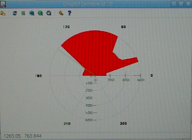
Figure 7 : Screen plot
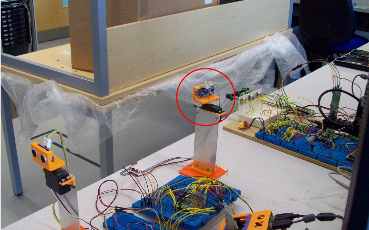
Figure 8 : Table
This program works, but the timing of the servo pulse does vary a little, resulting in servo jitter i.e. delays in receiving the ultrasonic signal, operating system calls, or just simply updating the mouse pointer position etc, means that the servo pulse is not the correct length or is not produced at the correct time, as shown in figure 9. A video of the software controlled servo is available here: (Video).
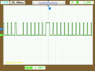
Figure 9 : Pulse jitter
To remove this jitter the servo can be controlled by dedicated hardware i.e. using a CPLD, as shown in figures 10 - 13. The Raspberry Pi tells the CPLD what position to turn the servo to, low level control is now done in hardware, therefore, any small changes in the software timings no longer affects the servo control pulse. This hardware was based on the following example: (Link) (Local). To further simplify the software, control of the ultrasonic sensor can also be passed to the CPLD. The Raspberry Pi now requests a distance measurement from the CPLD which returns a 7 bit value. Again all low level control / timing is performed in hardware on the CPLD, a simple state machine, coded in VHDL.
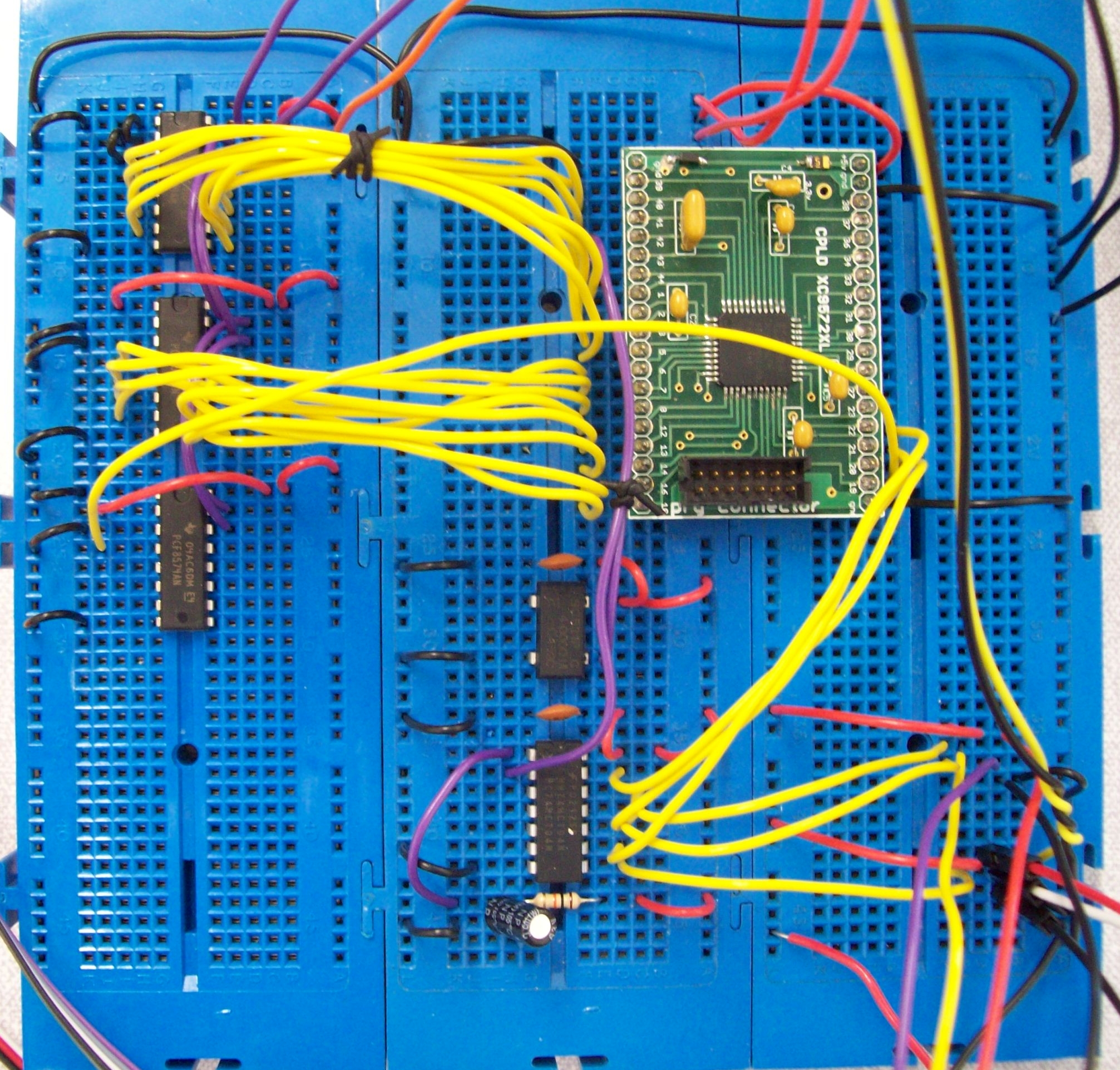
Figure 10 : Hardware system interface
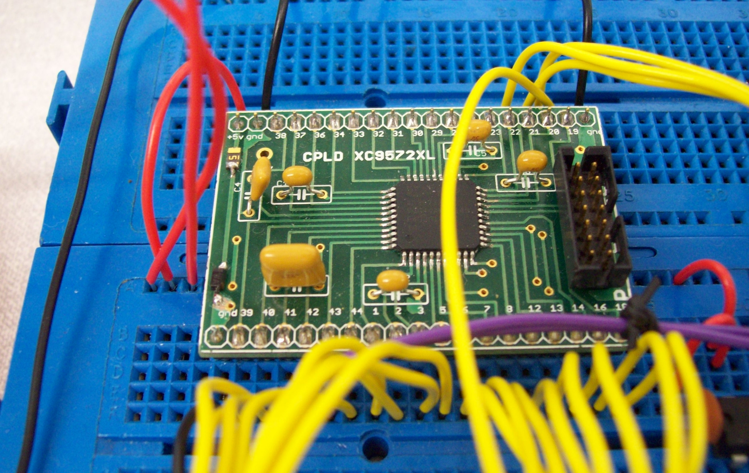
Figure 11 : CPLD
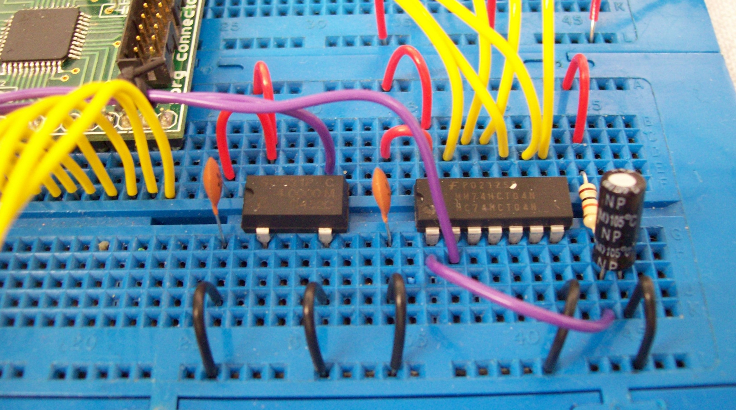
Figure 12 : Clock (4MHz) and Buffer
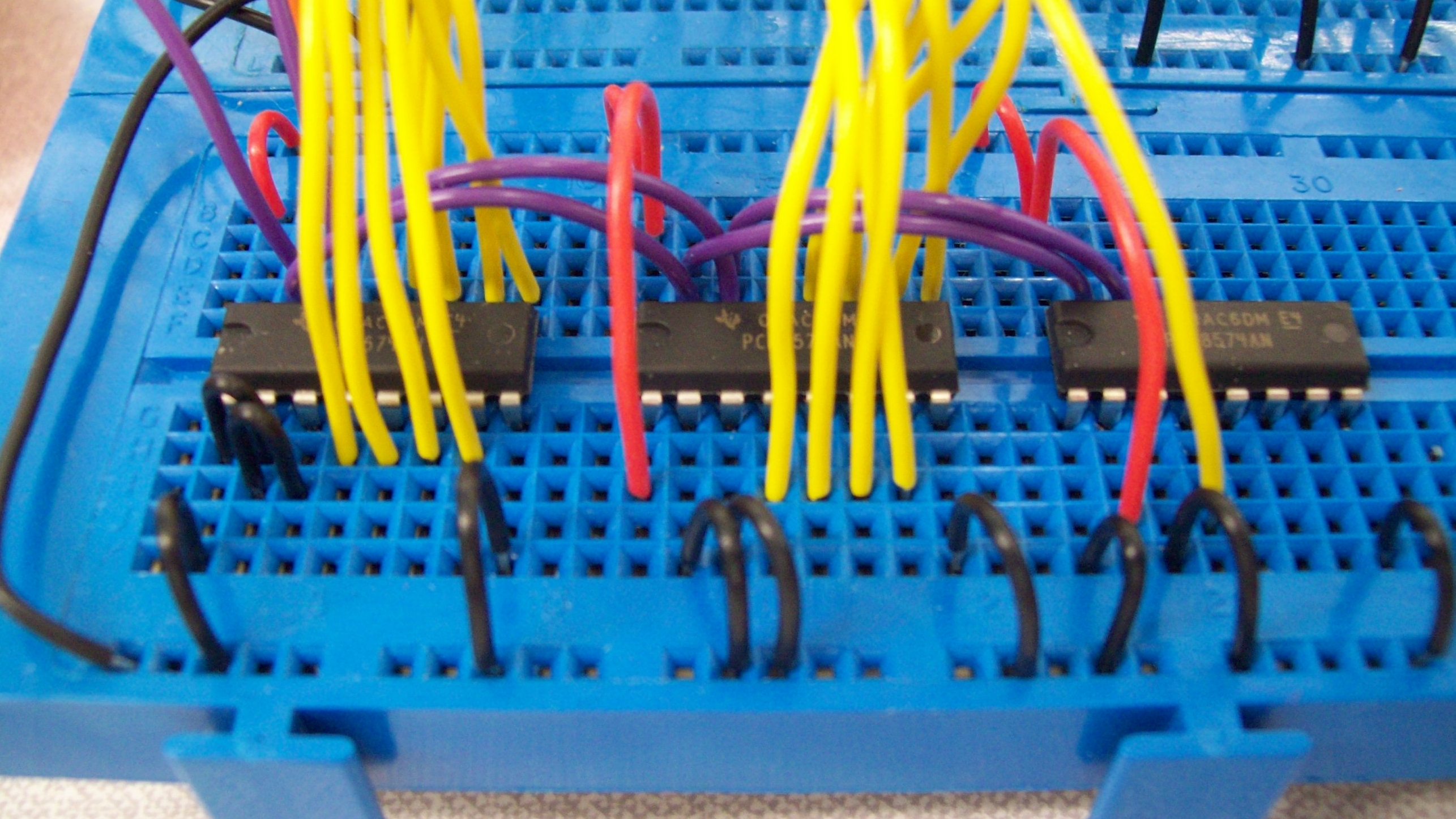
Figure 13 : I2C interface
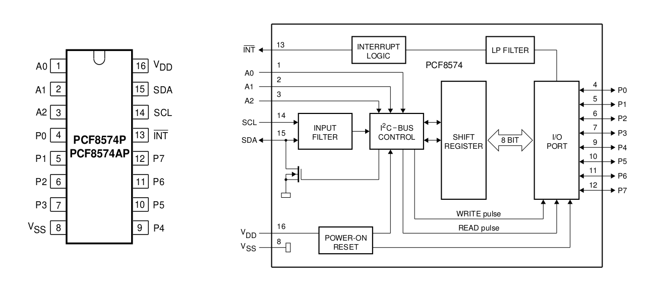
Figure 14 : I2C interface IC
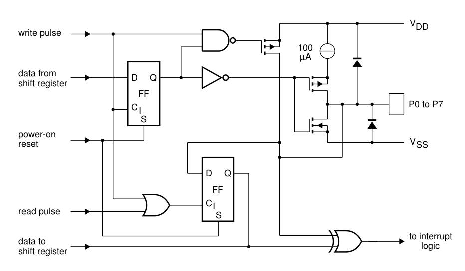
Figure 15 : I2C interface internals
To allow the Raspberry Pi to communicate to the CPLD it needs a data link. The simplest way to do this is to used three PCF8574 I2C 8bit IO expanders (Local), as shown in figures 13 - 15. Two are set up as outputs (servo position and US sensor control) and one as an input (US sensor data), the Raspbery Pi can then read or write to these I2C mapped addresses. Connected to these parallel ports is the CPLD as shown in figure 16 - 17. This operates from a 4MHz clock, with an internal clock divider generating the timing signals needed for each hardware subsystem. Individual VHDL files and the complete CPLD ISE project is available here:
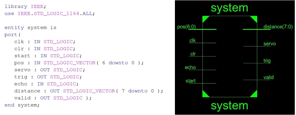
Figure 16 : Top Level Hardware Controller, VHDL (left), Symbol (right)
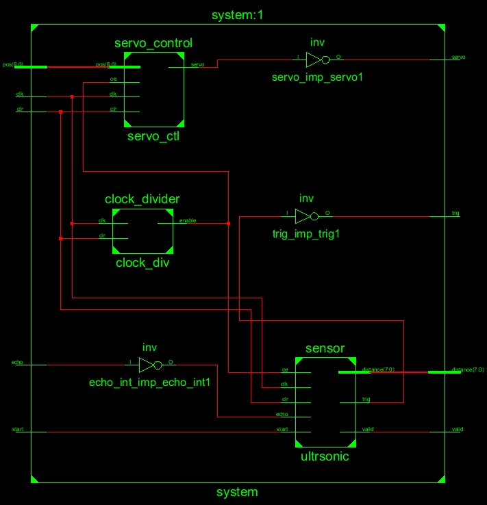
Figure 17 : Hardware Controller
Top level control is implemented in another python program, shown below:
import smbus
import time

POS_I2C_ADDR = 0x38
DIS_I2C_ADDR = 0x39
CTL_I2C_ADDR = 0x3A

bus = smbus.SMBus(1)

pos = 0
pos_prev = 31
direction = True

# Distance (37)

b = [0,0,0,0,0,0,0,0,0,0,0,0,0,0,0,0,0,0,0,0,0,0,0,0,0,0,0,0,0,0,0,0,0,0,0,0,0]
c = [0,0,0,0,0,0,0,0,0,0,0,0,0,0,0,0,0,0,0,0,0,0,0,0,0,0,0,0,0,0,0,0,0,0,0,0,0]

bus.write_byte(DIS_I2C_ADDR, 0xFF)

while True:
	# Trigger TX

	bus.write_byte(CTL_I2C_ADDR, 0x01)
	bus.write_byte(CTL_I2C_ADDR, 0x00)

	# Time to send start = 2 x 50us
	# Start pulse 200us
	# Max RX wait 10ms
	# Software delay 0.1s = 100ms

	time.sleep(0.1)

	# Time to read 50us

	data = bus.read_byte(DIS_I2C_ADDR)

	# print "Distance: " + str(data)

	# Speed of sound 340m/s, clock 64KHz = 15us
	# 1 sec = 340,000mm
	# 1 tick = 2.5mm

	distance = float(data) * 2.5

	# Max distance = 255 x 2.5 = 638mm

	if distance > 600:
		distance = 600

	# print "Distance: " + str(data)

	file = open('plot.dat', 'w')
	outputString = "\n"

	c[pos] = 600
	c[pos_prev] = 0

	for i in range(0,31):
		if pos == i:
			b[i] = distance

		outputString = outputString + str(i*6) + "\t" + str(b[i]) + "\t" + str(c[i]) + "\n"

	file.write(outputString)
	file.close

	pos_prev = pos

	if direction:
		pos = pos + 1
	else:
		pos = pos - 1

	if pos == 31:
		direction = False
		pos = 29

	if pos < 0:
		direction = True
		pos = 1

	# Print Angle
	print "Angle: " + str( pos ) + " Distance: " + str(data)

	bus.write_byte(POS_I2C_ADDR, int(float(pos) * 3.5))
	time.sleep(0.2)
As servo control is implemented in dedicated hardware, timing resolution can be more accurately controlled, allowing more readings to be taken during a scan. A video of the hardware controlled servo is available here: (Video).
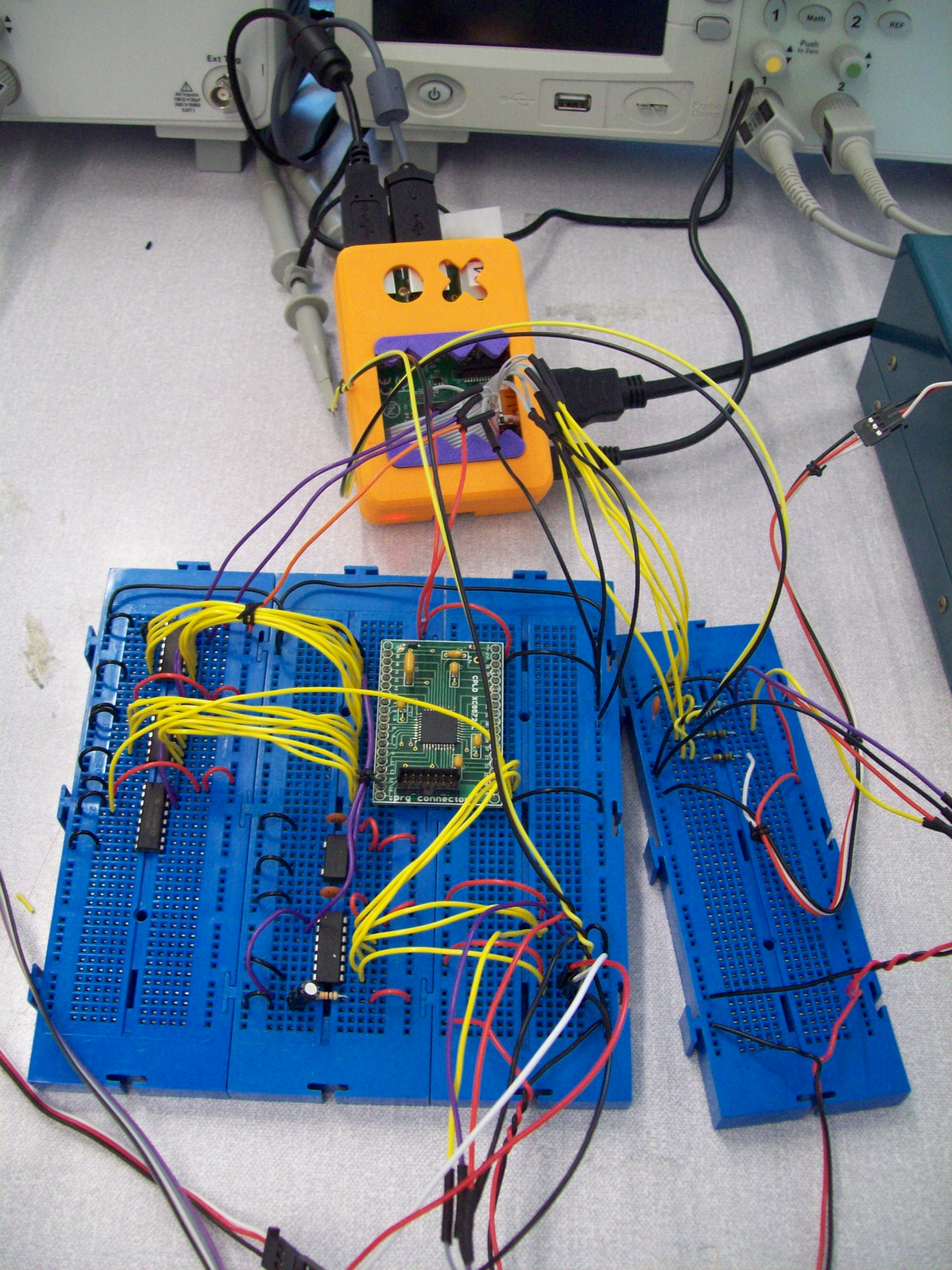
Figure 18 : System
The GNUplot display was a bit of a bodge, a quick and dirty solution. Finally got around to getting a nicer GUI working using Tkinter. Do confess GUIs are not my thing, to simplify the job went for a simple gif background (shown in figure 19) and canvas + lines.
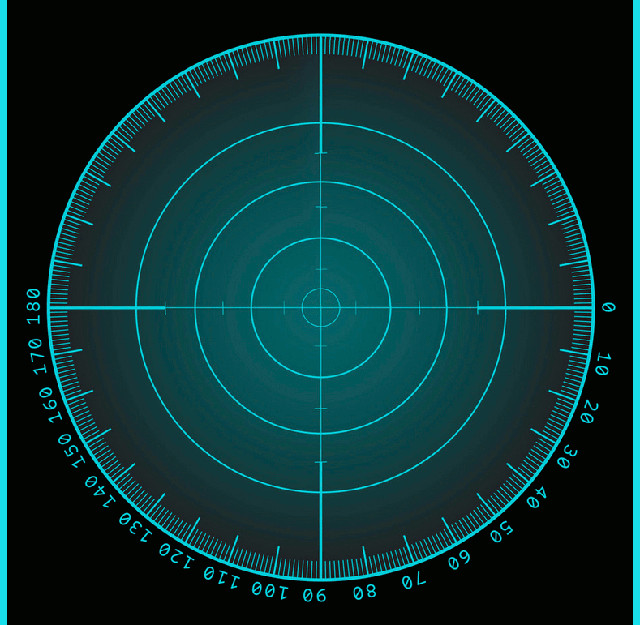
Figure 19 : GIF background
Test code is below, current reading is displayed in green, readings recorded during the current sweep are a light blue, readings recorded on the previous sweep a dark blue. A video of the software display random test data value is available here: (Video).
import Tkinter as tk
import math
import random

canvasWidth = 860
canvasHeight = 860

canvasCenterX = (canvasWidth/2)
canvasCenterY = (canvasHeight/2)

centerRadius = 10
angleOffset = 90

lineWidth = 3
lineLength = 300

lineNumber = 0
lineObjects = []

colourScale = [(0,255,0), (0, 208, 226), (0,190,207), (0,170,188), (0,150,162), (0,130,142), (0,110,121), (0,90,100), (0,75,75), (0,50,50)]

clockwise = True
anticlockwise = False

# Init measurement array (36)

measurement = []
for i in range(0, 185, 5):
	ran_number = random.random()
	distance =  int(ran_number*300)
	measurementData = (i, distance)
	measurement.append( measurementData )

def updateDisplay():
	global lineNumber, lineObjects, clockwise, anticlockwise, measurement

	#print len(measurement), lineNumber

	angle = measurement[lineNumber][0]
	length = measurement[lineNumber][1]

	dx = length * math.sin(math.radians(angleOffset - angle))
	dy = length * math.cos(math.radians(angleOffset - angle))

	colour = '#%02x%02x%02x' % colourScale[0]
	lineObjects.append(canvas.create_line(canvasCenterX, canvasCenterY, dx+canvasCenterX, dy+canvasCenterY, width=lineWidth, fill=colour))

	if lineNumber != 0:
		if clockwise:
			canvas.delete(lineObjects[lineNumber-1])

			angle = measurement[lineNumber-1][0]
			length = measurement[lineNumber-1][1]

			dx = length * math.sin(math.radians(angleOffset - angle))
			dy = length * math.cos(math.radians(angleOffset - angle))

			colour = '#%02x%02x%02x' % colourScale[1]
			lineObjects[lineNumber-1] = canvas.create_line(canvasCenterX, canvasCenterY, dx+canvasCenterX, dy+canvasCenterY, width=lineWidth, fill=colour)
		else:
			if lineNumber < (len(measurement)-1):
				canvas.delete(lineObjects[lineNumber+1])

				angle = measurement[lineNumber+1][0]
				length = measurement[lineNumber+1][1]

				dx = length * math.sin(math.radians(angleOffset - angle))
				dy = length * math.cos(math.radians(angleOffset - angle))

				colour = '#%02x%02x%02x' % colourScale[1]
				lineObjects[lineNumber+1] = canvas.create_line(canvasCenterX, canvasCenterY, dx+canvasCenterX, dy+canvasCenterY, width=lineWidth, fill=colour)

	if clockwise:
		lineNumber +=1
	else:
		lineNumber -=1

	if ((lineNumber == len(measurement)) and clockwise) or ((lineNumber == -1) and anticlockwise):
		for i in range(0, len(lineObjects)):
			canvas.delete(lineObjects[i])

		lineObjects = []
		for i in range(0, len(measurement)):
			angle = measurement[i][0]
			length = measurement[i][1]

			dx = length * math.sin(math.radians(angleOffset - angle))
			dy = length * math.cos(math.radians(angleOffset - angle))

			colour = '#%02x%02x%02x' % colourScale[5]
			lineObjects.append(canvas.create_line(canvasCenterX, canvasCenterY, dx+canvasCenterX, dy+canvasCenterY, width=lineWidth, fill=colour))

		if clockwise:
			clockwise = False
			anticlockwise = True
			lineNumber -=1
		else:
			clockwise = True
			anticlockwise = False
			lineNumber = 0

		measurement =[]
		for i in range(0, 185, 5):
			ran_number = random.random()
			distance =  int(ran_number*300)
			measurementData = (i, distance)
			measurement.append( measurementData )

	root.after(200, updateDisplay)

root = tk.Tk()
frame = tk.Frame(root)
frame.pack()

canvas = tk.Canvas(frame, width=canvasWidth, height=canvasHeight, bg='black')
canvas.pack(expand=tk.YES, fill=tk.BOTH)

photo=tk.PhotoImage(file='background2.gif')
canvas.create_image(35, 50, image=photo, anchor=tk.NW)

colour = '#%02x%02x%02x' % colourScale[8]
canvas.create_oval(canvasCenterX-centerRadius, canvasCenterY-centerRadius, canvasCenterX+centerRadius, canvasCenterY+centerRadius, width=0, fill=colour)

root.after(0, updateDisplay)
root.mainloop()

This work is licensed under a Creative Commons Attribution-NonCommercial-NoDerivatives 4.0 International License.
Contact details: email - mike.freeman@york.ac.uk, telephone - 01904 32(5473)
Back