Meta-analysis is the combination of data from several studies to produce a single estimate. From the statistical point of view, meta-analysis is a straightforward application of multifactorial methods. We have several studies of the same thing, which might be clinical trials or epidemiological studies, perhaps carried out in different countries. Each trial gives us an estimate of an effect. We assume that these are estimates of the same global population value. We check the assumptions of the analysis, and, if these assumptions are satisfied, we combine the separate study estimates to make a common estimate. This is a multifactorial analysis, where the treatment or risk factor is one predictor variable and the study is another, categorical, predictor variable.
The main problems of meta-analysis arise before we begin the analysis of the data. First, we must have a clear definition of the question so that we only include studies which address this. For example, if we want to know whether lowering serum cholesterol reduces mortality from coronary artery disease, we would not want to include a study where the attempt to lower cholesterol failed. On the other hand, if we ask whether dietary advice lowers mortality, we would include such a study. Which studies we include may have a profound influence on the conclusions (Thompson 1993). Second, we must have all the relevant studies. A simple literature search is not enough. Not all studies which have been started are published; studies which produce significant differences are more likely to be published than those which do not (e.g. Pocock and Hughes 1990; Easterbrook et al. 1991). Within a study, results which are significant may be emphasized and parts of the data which produce no differences may be ignored by the investigators as uninteresting. Publication of unfavourable results may be discouraged by the sponsors of research. Researchers who are not native English speakers may feel that publication in the English language literature is more prestigious as it will reach a wider audience, and so try there first, only publishing in their own language if they cannot publish in English. The English language literature may thus contain more positive results than do other literatures. The phenomenon by which significant and positive results are more likely to be reported, and reported more prominently, than non-significant and negative ones is called publication bias. Thus we must not only trawl the published literature for studies, but use personal knowledge of ourselves and others to locate all the unpublished studies. Only then should we carry out the meta-analysis.
When we have all the studies which meet the definition, we combine them to get a common estimate of the effect of the treatment or risk factor. We regard the studies as providing several observations of the same population value. There are two stages in meta-analysis. First we check that the studies do provide estimates of the same thing. Second, we calculate the common estimate and its confidence interval. To do this we may have the original data from all the studies, which we can combine into one large data file with study as one of the variables, or we may only have summary statistics obtained from publications.
If the outcome measure is continuous, such as mean fall in blood pressure, we can check that subjects are from the same population by analysis of variance, with treatment or risk factor, study, and interaction between them in the model. Multiple regression can also be used, remembering that study is a categorical variable and dummy variables are required. We test the treatment times study interaction in the usual way. If the interaction is significant this indicates that the treatment effect is not the same in all studies, and so we cannot combine the studies. It is the interaction which is important. It does not matter much if the mean blood pressure varies from study to study. What matters is whether the effect of the treatment on blood pressure varies more than we would expect. We may want to examine the studies to see whether any characteristic of the studies explains this variation. This might be a feature of the subjects, the treatment or the data collection. If there is no interaction, then the data are consistent with the treatment or risk factor effect being constant. This is called a fixed effects model (see Section 10.12). We can drop the interaction term from the model and the treatment or risk factor effect is then the estimate we want. Its standard error and confidence interval are found as described in Section 17.2. If there is an interaction, we cannot estimate a single treatment effect. We can think of the studies as a random sample of the possible trials and estimate the mean treatment effect for this population. This is called the random effects model (Section 10.12). The confidence interval is usually much wider than that found using the fixed effect model.
If the outcome measure is dichotomous, such as survived or died, the estimate of the treatment or risk factor effect will be in the form of an odds ratio (Section 13.7). We can proceed in the same way as for a continuous outcome, using logistic regression (Section 17.8). Several other methods exist for checking the homogeneity of the odds ratios across studies, such as Woolf's test (see Armitage and Berry 1994) or that of Breslow and Day (1980). They all give similar answers, and, since they are based on different large-sample approximations, the larger the study samples the more similar the results will be. Provided the odds ratios are homogeneous across studies, we can then estimate the common odds ratio. This can be done using the Mantel-Haenszel method (see Armitage and Berry 1994) or by logistic regression.
For example, Glasziou and Mackerras (1993) carried out a meta-analysis of vitamin A supplementation in infectious disease. Their data for five community studies are shown in the Table:
| Dose regime | Vitamin A | Controls | |||
|---|---|---|---|---|---|
| deaths | number | deaths | number | ||
| 1. | 200,000 IU six-monthly | 101 | 12,991 | 130 | 12,209 |
| 2. | 200,000 IU six-monthly | 39 | 7,076 | 41 | 7,006 |
| 3. | 8,333 IU weekly | 37 | 7,764 | 80 | 7,755 |
| 4. | 200,000 IU four-monthly | 152 | 12,541 | 210 | 12,264 |
| 5. | 200,000 IU once | 138 | 3,786 | 167 | 3,411 |
We can obtain odds ratios and confidence intervals as described in Section 13.7:
| Study | Odds ratio | 95% confidence interval |
|---|---|---|
| 1 | 0.73 | 0.56 to 0.95 |
| 2 | 0.94 | 0.61 to 1.46 |
| 3 | 0.46 | 0.31 to 0.68 |
| 4 | 0.70 | 0.57 to 0.87 |
| 5 | 0.73 | 0.58 to 0.93 |
The common odds ratio can be found in several ways. To use logistic regression, we regress the event of death on vitamin A treatment and study. I shall treat the treatment as a dichotomous variable, set to 1 if treated with vitamin A, 0 if control. Study is a categorical variable, so we create dummy variables study1 to study4, which are set to one for studies 1 to 4 respectively, and to zero otherwise. We test the interaction by creating another set of variables, the products of study1 to study4 and vitamin A. Logistic regression of death on vitamin A, study and interaction gives a chi-squared statistic for the model of 496.99 with 9 degrees of freedom, which is highly significant. Logistic regression without the interaction terms gives 490.33 with 5 degrees of freedom The difference is 496.99 - 490.33 = 6.66 with 9-5 = 4 degrees of freedom, which has P = 0.15, so we can drop the interaction from the model. The adjusted odds ratio for vitamin A is 0.70, 95% confidence interval 0.62 to 0.79, P<0.0001.
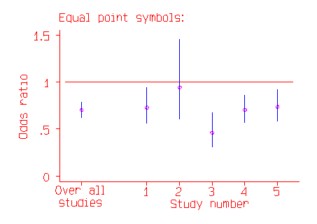
The odds ratios and their confidence intervals are shown in the following figure. The confidence interval is indicated by a line, the point estimate of the odds ratio by a circle.

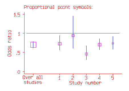
In the above picture the most important trial appears to be Study 2, with the widest confidence interval. In fact, it is the study with the least effect on the whole estimate, because it is the study where the odds ratio is least well estimated. In the second picture, the odds ratio is indicated by the middle of a square.

The area of the square is proportional to the number of subjects in the study. This now makes Study 2 appear relatively unimportant, and makes the overall estimate stand out.
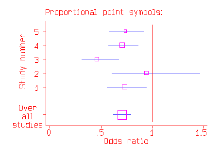
There many variants on this style of graph, which is sometimes called a forest diagram. The graph is often shown with the studies on the vertical axis and the odds ratio or difference in mean on the horizontal axis:

The combined estimate of the effect may be shown as a lozenge or diamond shape and for odds ratios a logarithmic scale is often employed.
Armitage, P. and Berry, G. (1994) Statistical Methods in Medical Research, 3rd Ed. Blackwell, Oxford.
Breslow, N.E. and Day, N.E. (1987) Statistical methods in cancer research. Volume II - the design and analysis of cohort studies IARC, Lyon.
Easterbrook. P.J., Berlin, J.A., Gopalan, R., and Mathews, D.R. (1991) Publication bias in clinical research. Lancet 337 867-72.
Glasziou, P.P. and Mackerras, D.E.M. (1993) Vitamin A supplementation in infectious disease: a meta-analysis. British Medical Journal 306 366-70.
Pocock, S.J. and Hughes, M.D. (1990) Estimation issues in clinical trials and overviews. Statistics in Medicine 9 657-71.
Thompson, S.G. (1993) Controversies in meta-analysis: the case of the trials of serum cholesterol reduction. Statistical methods in medical research 2 173-92.
Back to An Introduction to Medical Statistics contents.
Back to Martin Bland's Home Page.
This page maintained by Martin Bland.
Last updated: 27 October, 2003.