In the study of measurement error, we sometimes find that the within-subject variation is not uniform but is proportional to the magnitude of the measurement. It is natural to estimate it in terms of the ratio within-subject standard deviation/mean, which we call the within-subject coefficient of variation.
In our British Medical Journal Statistics Note on the subject, Measurement error proportional to the mean, Doug Altman and I described how to calculate this using a logarithmic method. We take logarithms of the data and then find the within-subject standard deviation. We take the antilog of this and subtract one to get the coefficient of variation.
Alvine Bissery, statistician at the Centre d'Investigations Cliniques, Hôpital européen Georges Pompidou, Paris, pointed out that some authors suggest a more direct approach. We find the coefficient of variation for each subject separately, square these, find their mean, and take the square root of this mean. We can call this the root mean square approach. She asked what difference there is between these two methods.
In practice, there is very little difference between these two ways of estimating within-subject coefficient of variation. They give very similar estimates.
This simulation, done in Stata, shows what happens. (The function invnorm(uniform()) gives a standard Normal random variable.)
. clear
Set sample size to 100.
. set obs 100
obs was 0, now 100
We generate true values for the variable whose measurement we are simulating.
. gen t=6+invnorm(uniform())
We generate measurements x and y, with error proportional to the true value.
. gen x = t + invnorm(uniform())*t/20
. gen y = t + invnorm(uniform())*t/20
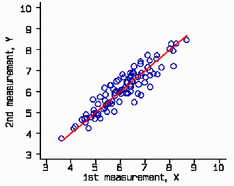
The simulated data look like this, shown as a scatter plot with the line of equality:

Calculate the within-subject variance for the natural scale values. (Within-subject variance is given by difference squared over 2 when we have pairs of subjects.)
. gen s2 = (x-y)^2/2
Calculate subject mean and s squared / mean squared, i.e. CV squared.
. gen m=(x+y)/2
. gen s2m2=s2/m^2
Calculate mean of s squared / mean squared.
. sum s2m2
Variable |     Obs        Mean   Std. Dev.       Min        Max
---------+-----------------------------------------------------
    s2m2 |     100    .0021519   .0030943   4.47e-07   .0166771
The within-subject CV is the square root of the mean of s squared / mean squared:
. disp sqrt(.0021519)
.04638858
Hence the within-subject CV is estimated to be 0.046 or 4.6%.
Now the log method. First we log transform.
. gen lx=log(x)
. gen ly=log(y)
Calculate the within-subject variance for the log values.
. gen s2l = (lx-ly)^2/2
. sum s2l
Variable |     Obs        Mean   Std. Dev.       Min        Max
---------+-----------------------------------------------------
     s2l |     100    .0021566    .003106   4.46e-07   .0167704
The within-subject standard deviation on the log scale is the square root of the mean within-subject variance. The CV is the antilog (exponent since we are using natural logarithms) minus one.
. disp exp(sqrt(.0021566))-1
.04753439
Hence the within-subject CV is estimated to be 0.048 or 4.8%. Compare this with the direct estimate, which was 4.6%. The two estimates are almost the same.
If we average the CV estimated for each subject, rather than their squares, we do not get the same answer.
Calculate subject CV and find the mean.
. gen cv=sqrt(s2)/m
. sum cv
Variable |     Obs        Mean   Std. Dev.       Min        Max
---------+-----------------------------------------------------
      cv |     100    .0361173   .0292567   .0006682   .1291399
This gives us the within-subject CV estimate = 0.036 or 3.6%. This is considerably smaller than the estimates by the root mean square method or the log method. The mean CV is not such a good estimate and we should avoid it.
Sometimes researchers estimate the within-subject CV using the mean and within-subject standard deviation for the whole data set. They estimate the within-subject standard deviation in the usual way, as if it were a constant. They then divide this by the mean of all the observations to give a CV. This appears to be a completely wrong approach, as it estimates a single value for a varying quantity. However, it often works remarkably well, though why it does I do not know. It works in this simulation:
. sum x y s2
Variable |     Obs        Mean   Std. Dev.       Min        Max
---------+-----------------------------------------------------
       x |     100    6.097301   1.012154    3.62283   8.696612
       y |     100    6.081827   1.000043   3.759932   8.447584
      s2 |     100    .0823188   .1212132   .0000193    .605556
The within-subject standard deviation is the square root of the mean of s2 and the overall mean is the average of the X mean and the Y mean. Hence the estimate of the within-subject CV is:
. disp  sqrt(.0823188)/( (6.097301 + 6.081827)/2)
.04711545
So this method gives the estimated within-subject CV as 0.047 or 4.7%. This can be compared to the estimates by the root mean squared CV and the log methods, which were 4.6% and 4.8%. Why this should be I do not know, but it works. I do not know whether it would work in all cases, so I do not recommend it.
We can find confidence intervals quite easily for estimates by either the root mean square method or the log method. For the root mean square method, this is very direct. We have the mean of the squared CV, so we use the usual confidence interval for a mean on this, then take the square root.
. sum s2m2
Variable |     Obs        Mean   Std. Dev.       Min        Max
---------+-----------------------------------------------------
    s2m2 |     100    .0021519   .0030943   4.47e-07   .0166771
The standard error is the standard deviation of the CVs divided by the square root of the sample size.
. disp .0030943/sqrt(100)
.00030943
The 95% confidence interval for the squared CV can be found by the mean minus or plus 1.96 standard errors. If the sample is small we should use the t distribution here. However, the squared CVs are unlikely to be Normal, so the CI will still be very approximate.
. disp .0021519 - 1.96*.00030943
.00154542
. disp .0021519 + 1.96*.00030943
.00275838
The square roots of these limits give the 95% confidence interval for the CV.
disp sqrt(.00154542)
.03931183
. disp sqrt(.00275838)
.05252028
Hence the 95% confidence interval for the within-subject CV by the root mean square method is 0.039 to 0.053, or 3.9% to 5.3%.
For the log method, we can find a confidence interval for the within-subject standard deviation on the log scale. The standard error is sw/root(2n(m-1)), where sw is the within-subject standard deviation, n is the number of subjects, and m is the number of observations per subject.
In the simulation, sw = root(0.0021566) = 0.0464392, n = 100, and m = 2.
Hence the standard error is 0.0464392/root(2 * 100 * (2-1)) = 0.0032837.
The 95% confidence interval is 0.0464392 - 1.96*0.0032837 = 0.0400031 to 0.0464392 + 1.96*0.0032837 = 0.0528753.
Finally, we antilog these limits and subtract one to give confidence limits for the CV: exp(0.0400031)-1 = 0.040814 and exp(0.0528753)-1 = 0.05429817, so the 95% confidence interval for the within-subject CV is 0.041 to 0.053, or 4.1% to 5.3%. These are slightly narrower than the root mean square confidence limits, but very similar.
I would conclude that either the root mean square method or the log method can be used.
Thanks to Garry Anderson for pointing out an error on this page.
Martin Bland
Back to frequently asked questions on the design and analysis of measurement studies.
Back to Martin Bland's home page.
This page maintained by Martin Bland.
Last updated: 16 October, 2006.