 D
D
One of the main purposes of making clinical measurements is to aid in diagnosis. This may be to identify one of several possible diagnoses in a patient, or to find people with a particular disease in an apparently healthy population. The latter is known as screening. In either case the measurement provides us with a test, which we may be able to compare later with a true diagnosis. The test may be based on a continuous variable and the disease indicated if this is above or below a given level, or it may be a qualitative observation such as carcinoma in situ cells on a cervical smear. In either case, we will call the test positive if it indicates the disease and negative if not, and the diagnosis positive if the disease is later confirmed, negative if not.
How do we measure the effectiveness of the test? Table 1 shows three artificial sets of test and diagnosis data.
| Test 1 | Disease diagnosis | Total | |
|---|---|---|---|
| positive | negative | ||
| positive | 4 | 5 | 9 |
| negative | 1 | 90 | 91 |
| Total | 5 | 95 | 100 |
| Test 2 | Disease diagnosis | Total | |
|---|---|---|---|
| positive | negative | ||
| positive | 0 | 0 | 0 |
| negative | 5 | 95 | 100 |
| Total | 5 | 95 | 100 |
| Test 3 | Disease diagnosis | Total | |
|---|---|---|---|
| positive | negative | ||
| positive | 2 | 0 | 2 |
| negative | 3 | 95 | 98 |
| Total | 5 | 95 | 100 |
We could take as an index of test effectiveness the proportion giving the true diagnosis from the test. For Test 1 in the example it is 94%. Now consider Test 2, which always gives a negative result. Test 2 will never detect any cases of the disease. We are now right for 95% of the subjects! However, the first test is useful, in that it detects some cases of the disease, and the second is not, so this is clearly a poor index.
We could use a coefficient of agreement, for example the number positive on both tests over the number positive on at least one test. For Test 1 this is 4/(4+5+1) = 0.4; for Test 2 it is 0/(0+0+5) = 0. This is better, but still not good enough. Compare Test 3, which has the same coefficient of agreement as Test 1, 2/(2+0+3) = 0.4.
For Cohen's kappa we get κ = 0.54, κ = 0.54, and κ = 0.56 for tests 1, 2, and 3 respectively. However, Test 3 is not as good as Test 1 in one respect: it only detects 2 of the 5 disease positives, compared to 4. On the other hand, it is a better test in another way: it does not diagnose as positive any disease negatives.
There is no one simple index which enables us to compare different tests in all the ways we would like. This is because there are two things we need to measure: how good the test is at finding disease positives, i.e. those with the condition, and how good the test is at excluding disease negatives, i.e. those who do not have the condition.
The indices conventionally employed to do this are:
sensitivity = number who are disease positive and test positive divided by number who are disease positive
and
specificity = number who are disease negative and test negative divided by number who are disease negative
In other words, the sensitivity is a proportion of disease positives who are test positive, and the specificity is the proportion of disease negatives who are test negatives.
For our three tests these are:
| Sensitivity | Specificity | |
|---|---|---|
| Test 1 | 0.80 | 0.95 |
| Test 2 | 0.00 | 1.00 |
| Test 3 | 0.40 | 1.00 |
Test 2, of course, misses all the disease positives and finds all the disease negatives, by saying all are negative. The difference between Tests 1 and 3 is brought out by the greater sensitivity of 1 and the greater specificity of 3. We are comparing tests in two dimensions. We can see that Test 3 is better than Test 2, because its sensitivity is higher and specificity the same. However, it is more difficult to see whether Test 3 is better than Test 1. We must come to a judgement based on the relative importance of sensitivity and specificity in the particular case. Sensitivity and specificity are often multiplied by 100 to give percentages. <> For a practical example, a remarkable number of alcoholics have evidence at X-ray of past rib fractures. We asked whether this would be of any value in the detection of alcoholism in patients. Among 74 patients with alcoholic liver disease, 20 had evidence of at least one past fracture on chest X-ray and 11 had evidence of bilateral or multiple fractures. In a control group of 181 patients with non-alcoholic liver disease or gastro-intestinal disorders, 6 had evidence of at least one fracture and 2 of bilateral or multiple fractures.
For any fractures as a test for alcoholism, the sensitivity was 20/74 = 0.27, and the specificity (181 – 6)/181 = 0.97. For bilateral or multiple fractures the sensitivity was 11/74 = 0.15 and the specificity was (181 – 2)/181 = 0.99. Hence both tests were very specific; very few non-alcoholics would be indicated as alcoholics by them. On the other hand, neither was very sensitive; many alcoholics would be missed. As might be expected, the more stringent test of bilateral or multiple fractures was more specific and less sensitive than the test of any fracture.
| Unstable angina | AMI | ||||||||
|---|---|---|---|---|---|---|---|---|---|
| 23 | 48 | 62 | 83 | 104 | 130 | 307 | 90 | 648 | |
| 33 | 49 | 63 | 84 | 105 | 139 | 351 | 196 | 894 | |
| 36 | 52 | 63 | 85 | 105 | 150 | 360 | 302 | 962 | |
| 37 | 52 | 65 | 86 | 107 | 155 | 311 | 1015 | ||
| 37 | 52 | 65 | 88 | 108 | 157 | 325 | 1143 | ||
| 41 | 53 | 66 | 88 | 109 | 162 | 335 | 1458 | ||
| 41 | 54 | 67 | 88 | 111 | 176 | 347 | 1955 | ||
| 41 | 57 | 71 | 89 | 114 | 180 | 349 | 2139 | ||
| 42 | 57 | 72 | 91 | 116 | 188 | 363 | 2200 | ||
| 42 | 58 | 72 | 94 | 118 | 198 | 377 | 3044 | ||
| 43 | 58 | 73 | 94 | 121 | 226 | 390 | 7590 | ||
| 45 | 58 | 73 | 95 | 121 | 232 | 398 | 11138 | ||
| 47 | 60 | 75 | 97 | 122 | 257 | 545 | |||
| 48 | 60 | 80 | 100 | 126 | 257 | 577 | |||
| 48 | 60 | 80 | 103 | 130 | 297 | 629 | |||
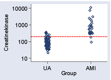
Figure 1 shows a scatter plot of CK against group.
Figure 1. Scatter diagram for the data of Table 2,
showing cut-off at 200
D
We wish to detect patients with AMI among patients who may have either condition and this measurement is a potential test, AMI patients tending to have high values. How do we choose the cut-off point?
The lowest CK in AMI patients is 90, so a cut-off below this will detect all AMI patients. Using 80, for example, we would detect all AMI patients, sensitivity = 1.00, but would also only have 42% of angina patients below 80, so the specificity = 0.42. We can alter the sensitivity and specificity by changing the cut-off point. Raising the cut-off point will mean fewer cases will be detected and so the sensitivity will be decreased. However, there will be fewer false positives, positives on test but who do not in fact have the disease, and the specificity will be increased. For example, if CK = 100 were the criterion for AMI, sensitivity would be 0.96 and specificity 0.62.
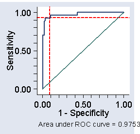
There is a trade-off between sensitivity and specificity. It can be helpful to plot sensitivity against specificity to examine this trade-off. This is called a receiver operating characteristic or ROC curve.
Figure 2. ROC curve for the data of Table 2,
showing cut-off at 200 and corresponding sensitivity and specificity
 D
D
(The name comes from telecommunications.) We often plot sensitivity against one minus specificity, as in Figure 2. We can see from Figure 1 that we can get both high sensitivity and high specificity if we choose the right cut-off. With 1-specificity less than 0.1, i.e. specificity greater than 0.9, we can get sensitivity greater than 0.9 also. In fact, a cut-off of 200 would give sensitivity = 0.93 and specificity = 0.91 in this sample.
These estimates will be biased, because we are estimating the cut-off and testing it in the same sample. We should check the sensitivity and specificity of this cut-off in a different sample to be sure.
The area under the ROC curve is often quoted (here it is 0.9753). It estimates the probability that a member of one population chosen at random will exceed a member of the other population. It can be useful in comparing different tests. In this study another blood test gave us an area under the ROC curve = 0.9825, suggesting that the test may be slightly better than CK.
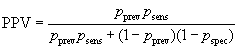
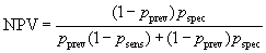
We can also estimate the probability that a subject who is test positive will also be a disease positive, called the positive predictive value or PPV. This depends on the prevalence of the condition. If our test and true diagnosis data are from a simple random sample of the population in which we are interested, we can estimate these as simple proportions. If this is not the case, the usual situation, we can calculate the PPV for any population prevalence.
Denote the sensitivity by psens, the specificity by pspec, and the prevalence by pprev.
The probability of being both disease positive and test positive is pprev×psens and the probability of being disease negative and test positive is (1 – pprev)× (1 – pspec). The total probability of being test positive is the sum of these: pprev×psens + (1 – pprev)×(1 – pspec). The positive predictive value is the proportion of test positives who are disease positives:
In screening situations the prevalence is almost always small and the PPV is low. Suppose we have a test which is both sensitive and specific, psens = 0.95 and pspec = 0.95, and the disease has prevalence pprev = 0.01 (1%). Then
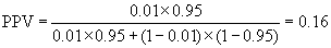
so only 16% of test positives would be disease positives.
The probability that a subject who is test negative will not have the disease is the negative predictive value or NPV.
It is usually high.
PPV and NPV are what we really want to know to interpret a test result, but they are properties of the test in a particular population, not just of the test.
There are other statistics quoted for tests, such as the odds ratio and the likelihood ratio, but they are beyond the scope of this course.
To Measurement in Health and Disease index.
To Martin Bland's M.Sc. index.
This page maintained by Martin Bland.
Last updated: 8 May, 2008.