Exercise: Alcohol consumption and sex

In the 2005 M.Sc. questionnaire, adult respondents were asked whether they were female or male and how much alcohol they usually consumed in a week.

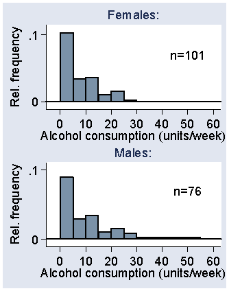
The distribution of reported alcohol consumption by sex is shown in the following graph:

d

The data may be summarised as follows:

	Number	Mean	SD
Female	101	6.6	6.4
Male	76	9.8	11.0

The difference in mean alcohol consumption, male minus female, is 3.2 units/week. The 95% confidence interval for the difference is 0.4 to 6.0 units/week, P = 0.02.

Question 1. What kind of graph is this and what are its main features?

Check suggested answer 1.

Question 2. What methods could be used to calculate the confidence interval for the difference in mean alcohol consumption? Which should we use here and why?

Check suggested answer 2.

Question 3. What does ‘The 95% confidence interval is 0.4 to 6.0 units/week’ mean and what conclusion could we draw from it?

Check suggested answer 3.

Question 4. What does ‘P=0.02’ mean and what can we conclude here?

Check suggested answer 4.

Respondents were asked whether they ever been diagnosed as having high blood pressure. The distribution of reported alcohol consumption by reported hypertension is shown in the following graph:

d

The data may be summarised as follows:

	Number	Mean	SD
Hypertensive	21	8.6	7.8
Normotensive	157	7.8	8.9

The difference in mean alcohol consumption, hypertensive minus normotensive, is 1.0 units/week. The 95% confidence interval for the difference in mean is –2.7 to +4.9 units/week, P = 0.6.

Question 5. In what way are these groups more difficult to compare than are men and women?

Check suggested answer 5.

6. If we accept the confidence interval and P value, what can we conclude about hypertension and alcohol consumption? What should we NOT conclude?

Check suggested answer 6.

To Applied Biostatistics index.

To Martin Bland's M.Sc. index.

To Martin Bland's home page.

This page maintained by Martin Bland.
Last updated: 1 November, 2006.

Back to top.