Coverage bias in the HadCRUT4 temperature record
Kevin Cowtan and Robert Way
FAQ
- Why did you base your work on the Hadley/CRU data?
-
Because Hadley are the only group to have addressed the sea surface temperature (SST) bias issue, a problem too complex for us to address.
more/less
Additionally, the Hadley dataset is the only version of the temperature record which has not already been subject to smoothing or interpolation. As a result it is the only dataset from which we could obtain realistic estimates of the spatial variability in the temperature data.
- How can the UAH satellite data be used to provide a global reconstruction when it doesn't cover the poles?
-
The satellite blind spot at the poles is very small and can easily be interpolated over - this is already done in the UAH data. We have validated our results against the International Arctic Buoy Program data and 3 weather models for the North Pole, and against the Amundsen Scott South Pole Station record, which lies at the centre of the Antarctic blind spot.
more/less
Check it for yourself
Run the makebias.csh and makehad4.csh scripts. Now, starting from the hybrid reconstruction (had4_1.0.dat), use masklat.py to remove the top and bottom 5 degrees of data. Use temp.py to calculate a temperature series. Finally use trend.py to determine the trend on the period 1997-2012. How does the trend compare to the full hybrid reconstruction?
Use the program nullfill.py to fill the polar holes with the mean value from the rest of the map, which does not affect the mean. Are the resulting maps realistic?
- Isn't the satellite data unreliable over Antarctica (hence RSS don't cover it)?
-
The satellite data does indeed show some interesting features over Antarctica - we hope to publish an update on this. However in holdout tests the hybrid approach provides a better reconstruction than kriging for every Antarctic station except for one.
more/less
While RSS omit the Antarctic in their satellite reconstructions, both UAH and NOAA include it. While there are clearly difficulties with the data, our results support this decision.
Check it for yourself
Run the makebias.csh, makehad4.csh and makecross1.csh scripts. Examine the files rmsd_1_krig.dat and rmsd_1_1.0.dat. The Antarctic stations are in the bottom few rows. Which method has more skill in reconstructing the omitted stations: Kriging or hybrid (s=1.0)?
Repeat this test for the land-only reconstruction in the had4-l directory. After reading our 30/10/2013 update, can you deduce what factors affect whether the satellite data helps or not?
- Is the use of the satellite data or infilling meaningful over the Arctic?
- We validate our reconstruction against both the International Arctic Buoy Program data, and against 3 weather models (Figure S5).
more/less
The problem with the Arctic ice pack is a lack of permanent weather stations against which to validate the results. The only source of in-situ observations are the IABP data to 1998 (Rigor et al, 2000). Our reconstruction reproduces the IABP data very well apart from 2 excursions around 1997/1998 and 1991/2. The month-on-month variation in our data shows good agreement with 3 weather models, which tend to support our reconstruction over the problem periods.
The 16 year trends are more difficult, because the IABP data does not cover this period. The weather models show somewhat different trends, suggesting that there are problems in modeling the central Arctic. Our reconstruction is more conservative than any of the 3 models over this period, and is closest to the ERA-interim model (Dee et al, 2011. See also papers by Screen et al).
The Arctic is sufficiently small that there is no significant difference between the kriging and hybrid reconstructions over this region.
- Dee et al. (2011). The ERA-Interim reanalysis: configuration and performance of the data assimilation system. Quarterly Journal of the Royal Meteorological Society, 137(656): 553-597.
- Rigor, I.G., Colony, R.L. and Martin, S. (2000). Variations in Surface Air Temperature Observations in the Arctic, 1979-97. Journal of Climate, 13(5): 896-914.
- Screen, J.A. and Simmonds, I. (2011). Erroneous Arctic Temperature Trends in the ERA-40 Reanalysis: A Closer Look. Journal of Climate, 24(10): 2620-2627.
- Screen, J.A., Deser, C. and Simmonds, I. (2012). Local and remote controls on observed Arctic warming. Geophysical Research Letters, 39(10).
- Is it meaningful to extrapolate temperatures across land/ocean boundaries?
-
There are problems with land/ocean boundaries, as we note in the paper. We validate our results against an alternative approach in our 30/10/2013 update.
more/less
Note that the in-situ temperature record aims to measure surface air temperature (and hence model-data comparisons are against T2m). The reason sea surface temperatures are used is that they provide a better estimate of air temperature over the oceans than Marine air temperatures, which have serious homogenization problems. However in the case of sea ice, the sea surface temperature is no longer a good measure of air temperature because the atmosphere is insulated from the ocean by a layer of snow and ice. This is confirmed by the IABP data and weather models.
The largest missing regions are either land or sea ice, and the nearest observations are from land stations. As a result reconstructing from the blended data provides a good approximation to reconstructing the domains separately. However reconstruction by domain has a number of benefits and we intend to adopt this approach in the long run.
Check it for yourself
Choose a cell in the sea ice in either the IABP or NCEP/NCAR data. Examine the variance of the cell over a fairly stable period, e.g. 1981-90. Now repeat the test for a land cell, either in the same data or in the CRUTEM4 data (had4-l directory). If possible examine both snow-covered and snow-free cells. Finally examine an ocean cell in the HadSST3 data (had4-o directory). What do the variances tell you?
- Do you use any form of atmospheric reanalysis in your data?
-
Atmospheric reanalysis data are not used in our global temperature reconstructions. We use them for validation where observational information is limited, and for uncertainty estimation.
more/less
In the context of the paper, we use atmospheric reanalysis products (NCEP and ECMWF) to help assess the degree of bias and latitudinal patterns in coverage bias within the HadCRUT4 dataset. Atmospheric reanalysis products are also used for comparison with our final results at both the global and regional scales including during comparisons with the International Arctic Buoy Program (IABP) dataset discussed by Rigor et al (2000).
In our results we show that atmospheric some reanalysis products perform reasonably well in determining surface air temperature (SAT) in the Arctic and Antarctic similar to results shown by Screen and Simmonds (2011), Screen et al (2012) and Screen and Simmonds (2012). In particular, the ERA-Interim atmospheric reanalysis dataset (Dee et al. 2011) provides the most realistic results in both Polar Regions and matches the regional patterns found in our study well. At mid-latitudes researchers should be cautious when using reanalysis products for assessing climate trends in air temperature.
- Dee et al. (2011). The ERA-Interim reanalysis: configuration and performance of the data assimilation system. Quarterly Journal of the Royal Meteorological Society, 137(656): 553-597.
- Rigor, I.G., Colony, R.L. and Martin, S. (2000). Variations in Surface Air Temperature Observations in the Arctic, 1979-97. Journal of Climate, 13(5): 896-914.
- Screen, J.A. and Simmonds, I. (2011). Erroneous Arctic Temperature Trends in the ERA-40 Reanalysis: A Closer Look. Journal of Climate, 24(10): 2620-2627.
- Screen, J.A., Deser, C. and Simmonds, I. (2012). Local and remote controls on observed Arctic warming. Geophysical Research Letters, 39(10).
- Screen, J.A. and Simmonds, I. (2012). Half-century air temperature change above Antarctica: Observed trends and spatial reconstructions. Journal of Geophysical Research, D16(27).
- How does your paper deal with uncertainties in the infilling?
-
The impact of uncertainties in the infilling on global temperature estimates is estimated by testing the skill of the method in reconstructing the NCEP/NCAR data, an approach derived from that used by the Met Office.
more/less
There are two kinds of uncertainties to consider: uncertainty in the temperature estimates for individual cells, and uncertainty in the global mean surface temperature. The latter is estimated by taking the reanalysis data, reducing coverage to match HadCRUT4, reconstructing a global map from the reduced map, and comparing the mean temperature to the original values. This does not require that the reanalysis data is correct, only that it is physically plausible.
Individual cell uncertainties do not figure in our work, but may be determined as an additional step in the kriging calculation. The program 'krig1v-var.py' does this calculation. Note that this code is only minimally tested and the resulting uncertainties may be inflated by a factor of √2 due to a missing factor of 2 in the (semi-)variogram calculation.
- Have you compared your data against climate model outputs?
-
No, however as we have noted the temperature changes are quite small and primarily affect the 15-16 year temperature trend.
more/less
Our work primarily addresses the impact of bias on recent temperature trends. Our results highlight the dangers of drawing conclusions from short term trends. This type of argument has dominated the public discourse, but is in our view a misleading approach to evaluating climate science.
The question of whether climate models predict the observations is a separate issue. This is a genuine scientific question which is not addressed by our work.
- Why did 1998 and 2010 show such large changes relative to other years? Could this be because of satellite sensitivity to ENSO??
-
The impact of coverage depends on the global distribution of temperature anomalies. Some atmospheric telleconnections (such as ENSO, Arctic Oscillation etc...) produce unique air temperature patterns which can change the distribution of warm temperature anomalies from being mostly in observed regions in HadCRUT4 to mostly in unobserved regions.
more/less
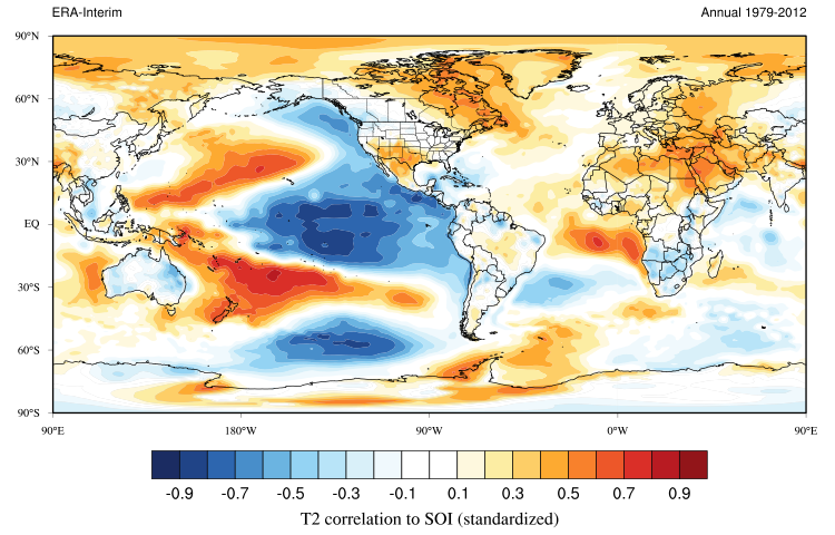
In the Cowtan and Way (2013) reconstruction the years 1998 and 2010 show the most change relative to the original HadCRUT4 dataset. The issues associated with reconstructing temperature patterns for these two years provide a great opportunity to show the impacts of coverage bias. Although 1998 and 2010 were both years that were characterized by warm air temperatures partly due to El Ninos they differed significantly in their synoptic patterns. In 1998 the very warm temperatures were at least partly caused by one of the most powerful El Ninos in recorded history (McPhaden, 1999). By contrast 2010 was characterized by a relatively moderate El Nino year but also the most negative Arctic Oscillation values in over 50 years (Cohen et al, 2010). The pattern of temperature change associated with El Nino shows that the response to ENSO events is strongest in the tropics and mid-to-low latitudes where observational data is the most complete (Figure 1). By contrast, the pattern of temperature change associated with the Arctic Oscillation is for the most part greatest in the high latitude regions of the Northern Hemisphere where observational coverage is fairly poor (Figure 2).
Considering the distinct synoptic patterns evident for both 1998 and 2010, we can see that temperatures in 1998 were warmer than 2010 for regions with the best observational coverage but were significantly lower than those in 2010 for regions with poor observational coverage such as the eastern Canadian Arctic (Figure 3). As a result of the coverage bias in the original HadCRUT4 the year 1998 was artificially warmer than it actually was and the year 2010 was cooler than in reality. This example shows clearly why improved observational coverage is important for understanding recent and past climate.

Figure 1
Figure 2
Figure 3Click to see full size versions Check it for yourself
Open the following .KMZ file in Google Earth showing the difference in temperature between 2010 and 1998 using ERA-Interim data. Consider the spatial distribution of these differences relative to this .KMZ file showing the typical extent of HadCRUT4 coverage over the period 1979-2012.
- McPhaden, M.J. (1999). Genesis and evolution of the 1997-98 El Nino. Science, 283(5404): 950-954.
- Cohen, J., Foster, J., Barlow, M., Saito, K. and Jones, J. (2010). Winter 2009-2010: A case study of an extreme Arctic Oscillation event. Geophysical Research Letters, 37.
- How does combining two datasets give a result with a trend greater than either?
-
We are not combining the surface and satellite data in the form of an average; we are using the spatial information from the satellite data in combination with the temporal information from the surface data.
more/less
The surface data comes from thousands of simple and standardised thermometers, and so has good temporal stability but uneven spatial coverage. The satellite data comes from a succession of single complex instruments, so while it has good geographical coverage, maintaining temporal stability is very challenging and different groups get different answers.
We use the spatial information from the satellite data to address the spatial incompleteness of the surface data. This could increase or decrease the trend in the surface data. The trend in the satellite data plays no part: This was a design decision of the method on the basis of the temporal stability issues. Adding an arbitrary time varying signal to the satellite data would not affect our results.
- Why do your corrections to HadCRUT4 show a discontinuity at the start of 2005?
-
Because January 2005 was much warmer than December 2004 in the central Arctic according to both observations and weather models.
more/less
The difference between our data and HadCRUT4 provides an estimate of coverage bias. Changes in coverage bias are controlled by two factors: Changes in the temperature contrast between the observed and unobserved regions, and changes in coverage. The two combine in a way analogous to the product rule in calculus.
There is a possible coverage issue: The most northerly station in the CRU data for the eastern hemisphere is POLARGMO. Data from this station are missing from Jan 2001 to Oct 2004 (SANNIKOVA STRAIT also has a gap in 2004). Without this station the central Arctic has rather less complete coverage, and as a result reverts naturally towards the global mean. Could this explain the jump? In this case no, the effect of removing this station is only about 0.01C.
The other alternative is temperature contrast. The MERRA weather model reanalysis does not assimilate weather station temperatures and so can be used as an independent test. The MERRA annual temperatures for our central Arctic test region are shown in the following figure, with 2004 highlighted in blue.
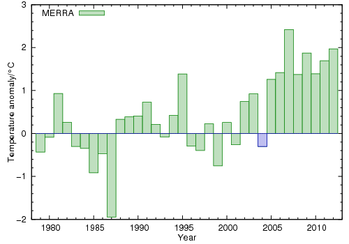
The MERRA temperature estimates for the central Arctic suggest that 2004 is over a degree cooler than 2005, and the jump from December 2004 to January 2005 is over 3°C. As a result the impact of leaving the Arctic out of the temperature data changes dramatically between the two months, creating a noticeable change in the HadCRUT4 bias. The step difference between our reconstruction and HadCRUT4 is an expected result of omitting the Arctic under these circumstances, and arises from coverage bias in the HadCRUT4 reconstruction.
The unobserved regions in the Antarctic are much larger and so also play a part even though the changes in the Antarctic are less extreme.
- Didn't this paper just set out to destroy the 'pause'?
-
The aim of the paper was to address a well known bias in the in situ temperature record.
more/less
This work was inspired back in 2011 by a desire to understand the divergence between the 3 main versions of the in situ temperature record. On inspecting the data it rapidly became obvious that the principal differences were due to coverage. Investigating the literature revealed that the issue was already well known.
The fact that trends starting around 1998 are unusually biased was unexpected. The discovery that the sea surface temperature bias was most significant over the same period was even more surprising. In retrospect however the connection is clear: The existence of these two biases impacting trends starting around 1998 have contributed to the identification of this period as a 'pause' in global warming.
- Why should we believe the paper when the authors have no prior publications on this subject?
-
Science is based on evidence, not belief. The paper should be evaluated on the basis of the evidence presented and consistency with other relevant evidence.
more/less
The problem is that evaluating the claims of a paper requires a similar level of expertise to writing it in the first place, so we often need to use other means to evaluate a paper. Whether it has passed peer-review is a useful one since, when it works, it means that other experts consider the work to be competently conducted. However experts are fallible, and a piece of research can be both competent and wrong for unexpected reasons.
The best test of the value of a piece of scientific work is to evaluate the response to the work over years or decades, with citations being a crude metric. For a more immediate evaluation, probably the best that can be achieved is to consult a range of experts with a good publication record in the subject of the work.