J. Martin Bland
Professor of Health Statistics
Department of Health Sciences
University of York
Talk to be presented at the Centre for Statistics in Medicine, Oxford
10 YEAR CELEBRATION
MEDICAL STATISTICS: MAKING A DIFFERENCE IN HEALTH CARE
Tuesday 20th September 2005
Measurement is a key part of clinical medicine and the development and evaluation of new methods of measurement is an important research activity. The misinterpretation of simple statistics is frequent in the analysis of such studies. This led to the development the limits of agreement approach, which has been widely adopted. Many problems remain and I shall illustrate some of these using a recent example concerning the measurement of blood glucose.
Given the theme 'Medical statistics: making a difference in health care', I thought I might start with a semi-quotation from John Cleese:
'What have the medical statisticians ever done for us?'
'Well, there's the clinical trials'
'Apart from the clinical trials, what have the medical statisticians ever done for us?'
and so on.
But I thought everybody might do that, so I start instead with a quotation from a most quotable man, Ralph Waldo Emerson (or some say Elbert Hubbard):
'If a man write a better book, preach a better sermon, or make a better mousetrap than his neighbour, tho' he build his house in the woods, the world will make a beaten path to his door.'
What made me think of this was that in July a paper which I wrote with Doug Altman on 'Statistical methods for assessing agreement between two methods of clinical measurement' exceeded 10,000 citations on the ISI Web of Science. It is also, to my complete amazement, the highest cited paper in the history of the Lancet (Sharp 2004) and one of the ten most highly cited statistical papers ever (Ryan and Woodall 2005).
I thought that this meeting would be a good oportunity to mark this surprising event, so I am going to tell you a little bit about how we came to write it, say something about what is happening now, and show you a recent example which illustrates several points about statistics and medicine. Misleading measures of agreement
For me, this began when a clinical colleague came into my office and showed me a paper.
'There's something wrong with this, but I don't know what it is', he said.
The paper (Keim et al. 1976) was a comparison of dye-dilution and impedance cardiography used to measure cardiac stroke volume. They used correlation coefficients between measurements by the two methods. They did this for a group of patients. For 20 of these patients, they made several repeated pairs of measurements on the same subject. They then calculated the correlation between repeated pairs of measurements by the two methods separately on each of these 20 patients. The 20 correlation coefficients ranged from -0.77 to 0.80, with one correlation being significant at the 5 per cent level. They concluded that the two methods did not agree because low correlations were found when the range of cardiac output was small, even though other studies covering a wide range of cardiac output had shown high correlations.
To a statistician, the reason for their findings is easy to see and is nothing to do with the measurement of stroke volume. If we take a very simple model and think of each measurement as the sum of the true value of the measured quantity and the error due to measurement, we have:
variance of true values = sT2
variance of measurement error, method A = sA2
variance of measurement error, method B = sB2
In the simplest model errors have expectation zero and are independent of one another and of the true value, so that
variance of method A = sA2 + sT2
variance of method B = sB2 + sT2
covariance = sT2
Hence the expected value of the sample correlation coefficient r is
Clearly ρ is less than one, and it depends only on the relative sizes of sT2, sA2 and sB2. If sA2 and sB2 are not small compared to sT2, the correlation will be small no matter how good the agreement between the two methods.
In the extreme case, when we have several pairs of measurements on the same individual, sT2 = 0 (assuming that there are no temporal changes), and so ρ = 0 no matter how close the agreement is.
I mentioned this to Doug and he said: 'I have come across exactly the same thing in the measurement of blood pressure.'
He produced the following table:
| Systolic pressure | Diastolic pressure | |||||
|---|---|---|---|---|---|---|
| sA | sB | r | sA | sB | r | |
| Laughlin et al. (1980) | ||||||
| 1 | 13.4 a | 15.3 a | 0.69 | 6.1 a | 6.3 a | 0.63 |
| 2 | 0.83 | 0.55 | ||||
| 3 | 0.68 | 0.48 | ||||
| 4 | 0.66 | 0.37 | ||||
| Hunyor et al. (1978) | ||||||
| 1 | 40.0 | 40.3 | 0.997 | 15.9 | 13.2 | 0.938 |
| 2 | 41.5 | 36.7 | 0.994 | 15.5 | 14.0 | 0.863 |
| 3 | 40.1 | 41.8 | 0.970 | 16.2 | 17.8 | 0.927 |
| 4 | 41.6 | 38.8 | 0.984 | 14.7 | 15.0 | 0.736 |
| 5 | 40.6 | 37.9 | 0.985 | 15.9 | 19.0 | 0.685 |
| 6 | 43.3 | 37.0 | 0.987 | 16.7 | 15.5 | 0.789 |
| 7 | 45.5 | 38.7 | 0.967 | 23.9 | 26.9 | 0.941 |
| a Standard deviations for four sets of data combined. | ||||||
Diastolic blood pressure varies less between individuals than does systolic pressure, so that we would expect to observe a worse correlation for diastolic pressures when methods are compared in this way. In two papers (Laughlin et al., 1980; Hunyor et al., 1978) presenting between them 11 pairs of correlations, this phenomenon was observed every time. It is not an indication that the methods agree less well for diastolic than for systolic measurements. This table provides another illustration of the effect on the correlation coefficient of variation between individuals. The sample of patients in the study of Hunyor et al. had much greater standard deviations than the sample of Laughlin et al. and the correlations were correspondingly greater.
The Institute of Statisticians was planning a conference on Health Statistics and we decided to submit a paper on this interesting phenomenon. Doug unearthed a couple more misleading cases.
In one, the mean gestational age of human babies measured by two methods were compared (Cater 1979). If there was no significant difference on a paired t test, the methods of measurement were deemed to agree.
In the other, regression was used. Carr et al. (1979) compared two methods of measuring the heart's left ventricular ejection fraction. These authors gave the regression line of one method, Teichholz, on the other, angiography. They noted that the slope of the regression line differed significantly from one and concluded that methods did not agree. The reasoning was that if the two methods agreed, a plot of one against the other should follow a line where the two measurements were equal, the line y = x, with slope 1 and intercept 0.
Both dependent and independent variables are measured with error, but the least squares regression line ignores the error in x. It estimates the mean y for a given observed x. The expected slope is
β = sT2/(sA2 + sT2)
and is therefore less than 1.
How much less than 1 depends on the amount of measurement error of the method chosen as independent.
The expected intercept is  , and as β < 1
and if we have perfect agreement we expect
, and as β < 1
and if we have perfect agreement we expect  , α > 0.
We thought that giving a talk saying that everybody was doing it wrong and then sitting down would fall a bit flat. We needed to propose a method that was right. We thought that one was obvious from elementary statistical methods. If we are interested in agreement, we want to know how far apart measurements by the two different methods might be. We therefore started with the differences between measurements on the same subject by two methods. We can calculate the mean and standard deviation of these differences. Then, provided the mean and standard deviation are constant and the differences have an approximately Normal distribution, 95% of such differences should lie between the mean minus 1.96 SD and mean plus 1.96 SD. We later called these the 95% limits of agreement.
We also pointed out that a line of equality or identity on the scatter plot was much more informative than the regression line:
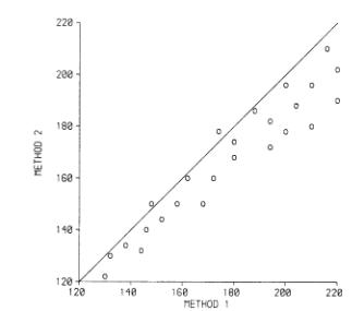
(These are the data of Daniel, 1978, which look fictitious to me. Daniel used them to illustrate the calculation of the correlation coefficient!) This example clearly shows that there is a bias, with the points lying on one side of the line. Even better is to plot the difference against the magnitude:
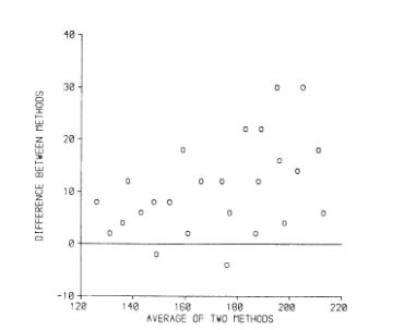
We suggested adding the 95% limits to the graph:
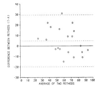
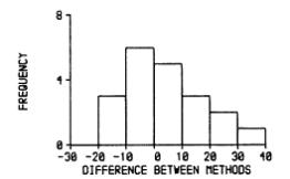
(data of Carr et al., 1979) and adding a histogram of the differences:
We thought that all these things were obvious and well-known, so when we gave our talk I expected someone to jump up and say something like 'Fisher did all this in 1933'. We did not claim any originality.
We presented the paper at the Institute of Statisticians conference in July 1981. To my surprise, nobody did say it had all been done before and nobody ever has, apart from claiming that plotting differences against average was not new. We entirely agree, it is in Peter Oldham's 1968 book Measurement in Medicine: The Interpretation of Numerical Data (Oldham 1968), for example. We were so concerned that this was all well-known to everyone but ourselves that we asked Michael Healy and David Cox whether they knew of it.
The paper was published in The Statistician in 1983 with authors Altman and Bland (Altman and Bland, 1983). I recall that we chose alphabetical order, agreeing that if we wrote another paper together we would swap. For both of us, this was our first statistical paper either in presentation or print.
Although the paper was well received by our statistical colleagues, it did not change anything and researchers carried on correlating. Several people suggested that we write a version for a medical audience, with a worked example. I collected some data according to our recommended design, two measurements by each method in random order, using a convenience sample of colleagues and family. I even got the peak expiratory flows of my parents and in-laws. We decided to aim high and sent this to the Lancet. To my amazement, they accepted it! I got a phone call from deputy editor David Sharp to tell me this, but saying that it should be shortened by 1/3. Sensing my inner groan, he said that the Lancet would do the shortening. Of course, we agreed. Doug recalls that this was on Christmas Eve, giving us a very nice present. When the reduced paper arrived I thought it was much better than our original effort. I persuaded him to put the confidence intervals back in and we were in business (Bland and Altman 1986).
The paper was a fantastic success, beyond my wildest dreams. In it we concentrated on the details of the limits of agreement approach, using that term for the first time. According to our initial authorship plan, the second paper was published under the names Bland and Altman, and so the method became known as 'the Bland Altman method'. Sorry, Doug!
Despite the high citation count, the same old things go on, often in papers which cite us. Bland and Altman (2003) describes some horrific examples from the radiological literature. They are horrific because people are drawing conclusions about methods of measurement which do not follow from their results. Good methods of measurement may be rejected, bad ones may be adopted as a result. Patients suffer.
I teach a masters' course on measurment in health and disease. Looking for some revision material for my students, I found a paper in the Medical Journal of Australia: 'Point-of-care testing of HbA(1c) and blood glucose in a remote Aboriginal Australian community' (Martin et al., 2005). The abstract included:
Results: Mean and median POC capillary glucose levels were 7.99 mmol/L and 6.25 mmol/L, respectively, while mean and median laboratory venous plasma glucose concentrations were 7.63 mmol/L and 5.35 mmol/L. Values for POC capillary HbA(1c) and laboratory HbA(1c) were identical: mean, 7.06%; and median, 6.0%. The correlation coefficient r for POC and laboratory results was 0.98 for glucose and 0.99 for HbA(1c). The mean difference in results was 0.36 mmol/L for glucose (95% Cl, 0.13-0.62; limits of agreement [LOA], −2.07 to 2.79 mmol/L; P = 0.007) and < 0.01% for HbA(1c) (95% Cl, −0.07% to 0.07%; LOA, −0.66% to 0.66%; P = 0.95), respectively.
This looked to have plenty of material and was on a clinical topic which should be fairly familiar to my students. It was especially attractive to me because I have spent a lot of time in God's Own Country over the last few years and I am diabetic who measures his own blood glucose every day. The paper was available on-line, so I had a look.
There I found this:
'This article was corrected on 27 May 2005 (the author Max K Bulsara, whose name had been inadvertently omitted from the manuscript, was added.)'
Max Bulsara is a statistician at the University of Western Australia and a mate, as the Aussies would say. This is how medical statisticians are treated!
The paper included the following figure:
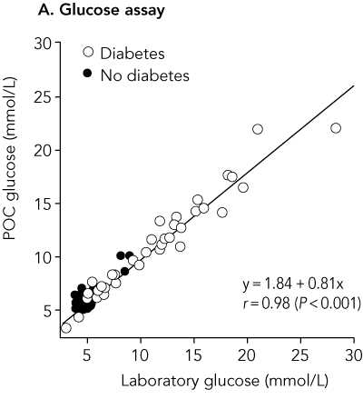
This graph is decorated with the usual useless regression equation, correlation coefficient, and P value. The last is testing the most implausible null hypothesis that these two measurements of glucose are not related. I suggested to Max Bulsara that a line of equality would be more informative:
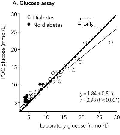
This clearly shows that for low glucose measurements capillary glucose overestimates laboratory glucose and for high glucose measurements capillary glucose underestimates laboratory glucose. Max told me that he had wanted to do this but that the lead author thought it made the graph look cluttered. Then he should get rid of the useless regression line!
The paper also included a difference versus mean plot:
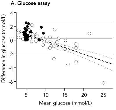
The horizontal lines on the plot are the 95% limits of agreement and the mean difference.
The simple 95% limits of agreement method relies on the assumptions that the mean and standard deviation of the differences are constant, i.e. that they do not depend on the magnitude of the measurement. In our original papers, we described the common situation where the standard deviation is proportional to the magnitude and described a method using a logarithmic transformation of the data. In our 1999 review paper (Bland and Altman 1999) we described a method for dealing with any relationship between mean and SD of differences and the magnitude of the measurement. (This was Doug Altman's idea, I can take no credit.)
If we estimate the crude 95% limits of agreement ignoring this relationship, we have mean difference = 0.3625 mmol/L, SD = 1.2357 mmol/L
crude lower limit = 0.3625 − 1.96 × 1.2357 = −2.06 mmol/L
crude upper limit = 0.3625 + 1.96 × 1.2357 = 2.78 mmol/L
From the difference versus mean plot, we can see that the limits do not fit the data well:
They are too wide at the low glucose end and too narrow at the high glucose end. The are correct in that they are expected to include 95% of differences (here 84/88 = 94.5%) but all the differences outside the limits are at one end and one of them is a long way outside.
A better fit can be found by using a regression method (Bland and Altman 1999). Max Bulsara sent me the data and I gave it a go. Regression of difference on average gives a highly significant relationship, P<0.001:
difference = 1.8799 − 0.1943 × average glucose
We can use this to model the relationship between mean difference and the magnitude of the blood glucose. If we take the residuals about this line, the differences between the observed difference and the difference predicted by the regression, we can use these to model the relationship between the standard deviation of the differences and the magnitude of the blood glucose.
What is the relationship between residuals and average? The regression will have mean zero and slope zero, by definition.
We calculate the absolute values of the residuals, without sign:
and then do regression of these on the differences.
This gives the following regression equation:
absolute residual = −0.02887 + 0.08525 × average glucose
which is statistically significant (P<0.001).
If we multiply these coefficients by  we get an equation to predict the standard deviation of the differences:
SD = −0.03618 + 0.1068 × average glucose
(For a mathematical proof of this see Bland, 2005). If we predict mean difference and standard deviation from these equations, we can estimate mean ± 1.96 SD for any magnitude of glucose:
lower limit = 1.8799 − 0.1943 × average glucose
− 1.96 × (−0.03618 + 0.1068 × average glucose)
= 1.8799 − 1.96 × (−0.03618)
+ (−0.1943 − 1.96× 0.1068) × average glucose
= 1.9508 − 0.4036 × average glucose
Similarly,
upper limit = 1.8799 + 1.96 × (−0.03618)
+ (−0.1943 + 1.96 × 0.1068) × average glucose
= 1.8090 + 0.0150 × average glucose
We can plot these limits on the difference versus mean plot:
The fit is greatly improved, particularly at the high glucose end. In practice, it would be sufficient to round these considerably, to between 2.0 − 0.4 × glucose and +1.8 mmol/L.
Changing established ideas is a long haul. In the analysis of measurement studies we are decades behind therapeutic or epidemiological studies.
When I came into medicine in 1972, I was surprised to learn that the randomised trial was a subject of hot debate, and regarded as a cutting edge innovation. This was 24 years after the publication of the MRC Streptomycin Trial (MRC 1948). It is only 19 years since our Lancet paper, so perhaps we should not be too discouraged.
I think statisticians have improved the quality of medical research tremendously. We did not do it on our own, of course, and it is the partnership between health professionals and statisticians which should get the credit. Sir Richard Doll, who died while I was writing this talk, and Sir Austin Bradford Hill together revolutionised epidemiological and clinical research.
I think that high profile medical research, that published in the major journals, is of much higher quality than when I began. There is still a lot to do, however, and the work continues.
I started with a quotation and I shall finish with two, both from William Blake (The Marriage of Heaven and Hell):
'The truth can never be told so as to be understood, and not be believ'd.'
'To create a little flower is the labour of ages.'
So if we keep at it, we should get there, but it might take a long time.
I thank Max Bulsara and David Martin for generously supplying their data. Most of all I thank Doug Altman for the best, most fruitful, and most enjoyable collaboration I have had.
Altman DG, Bland JM. (1983) Measurement in medicine: the analysis of method comparison studies. The Statistician 32, 307-317. (PDF file of Altman and Bland, 1983.)
Bland JM. (2005).
The Half-Normal distribution method for measurement error: two case studies.
(Unpublished talk available on
http://www-users.york.ac.uk/~mb55/talks/halfnor.pdf.)
Bland JM, Altman DG. (1986)
Statistical methods for assessing agreement between two methods of clinical measurement.
Lancet i, 307-310.
(Web copy of Bland and Altman, 1986.)
Bland JM, Altman DG. (1999) Measuring agreement in method comparison studies.
Statistical Methods in Medical Research 8, 135-160.
Bland JM, Altman DG. (2003) Applying the right statistics: analyses of measurement studies.
Ultrasound in Obstetrics & Gynecology 22, 85-93.
(Talk on which Bland and Altman 2003 was based.)
Carr, K. W., Engler, R. L., Forsythe, J. R., Johnson, A. D. and Gosink, B. (1979).
Measurement of left ventricular ejection fraction by mechanical cross-sectional echocardiography.
Circulation 59, 1196-1206.
Cater, J. I. (1979).
Confirmation of gestational age by external physical characteristics (total maturity score).
Archives of Disease in Childhood 54, 794-5.
Daniel, W. W. (1978).
Biostatistics: a Foundation for Analysis in the Health Sciences, 2nd edn. Wiley, New York.
Hunyor, S. M., Flynn, J. M. and Cochineas, C. (1978).
Comparison of performance of various sphygmomanometers with intra-arterial blood-pressure readings.
British Medical Journal 2, 159-62.
Keim, H. J., Wallace, J. M., Thurston, H., Case, D. B., Drayer, J. I. M. and Laragh, J. H. (1976).
Impedance cardiography for determination of stroke index.
Journal of Applied Physiology 41, 797-9.
Laughlin, K. D., Sherrard, D. J. and Fisher, L. (1980).
Comparison of clinic and home blood-pressure levels in essential hypertension and variables
associated with clinic-home differences.
Journal of Chronic Diseases 33, 197-206.
Martin DD, Shephard MDS, Freeman H, Bulsara MK, Jones TW, Davis EA, Maguire GP. (2005)
Point-of-care testing of HbA(1c) and blood glucose in a remote Aboriginal Australian community.
Medical Journal of Australia 182: 524-527.
MRC (1948)
Streptomycin treatment of pulmonary tuberculosis.
British Medical Journal 2, 769-82.
Oldham PD. (1968)
Measurement in Medicine: The Interpretation of Numerical Data.
English Universities Press, London.
Ryan TP and Woodall WH. (2005)
The most-cited statistical papers.
Journal of Applied Statistics 32, 461-474.
Sharp D. (2004) As we said...
Lancet 364 744.
Back to Some full length papers and talks.
Back to Martin Bland's Home Page.
This page is maintained by Martin Bland.
Last updated: 24 August, 2004.