 to
to
 .
.
We use sensitivity and specificity when we are concerned with the diagnosis of particular diseases. In this lecture we look at it the other way round and ask what values measurements on normal, healthy people are likely to have. There are difficulties in doing this. Who is 'normal' anyway? In the UK population, almost everyone has hard fatty deposits in their coronary arteries, which result in death for many of them. Very few Africans have this; they die from other causes. So it is normal in the UK to have an abnormality. We usually say that normal people are the apparently healthy members of the local population. We draw a representative sample of these and make the measurement on them.
The next problem is to estimate the set of values. If we use the range of the observations, the difference between the two most extreme values, we can be fairly confident that if we carry on sampling we will eventually find observations outside it, and the range will get bigger and bigger. To avoid this we use a range between two quantiles, usually the 2.5 centile and the 97.5 centile, which is called the normal range, 95% reference range or 95% reference interval. This leaves 5% of normals outside the 'normal range', which is the set of values within which 95% of measurements from apparently healthy individuals will lie.
A third difficulty comes from confusion between 'normal' as used in medicine and 'Normal distribution' as used in statistics. This has led some people to develop approaches which say that all data which do not fit under a Normal curve are abnormal! Such methods are simply absurd, there is no reason to suppose that all variables follow a Normal distribution. The term 'reference interval', which is becoming widely used, has the advantage of avoiding this confusion. However, the most commonly used method of calculation rests on the assumption that the variable follows a Normal distribution.
In general, most observations fall within two standard deviations
of the mean.
For a Normal distribution, 95% of observation are within these
limits with 2.5% below the lower limit and 2.5% above the upper limit.
(To be more precise, we should say ±1.96 rather than 2,
but the difference is tiny.)
If we estimate the mean and standard deviation of data from a
Normal population we can estimate the reference interval as
 to
to
 .
.
Consider the data of Table 1, FEV1 measured from 57 male students.
| 2.85 | 3.19 | 3.50 | 3.69 | 3.90 | 4.14 | 4.32 | 4.50 | 4.80 | 5.20 |
| 2.85 | 3.20 | 3.54 | 3.70 | 3.96 | 4.16 | 4.44 | 4.56 | 4.80 | 5.30 |
| 2.98 | 3.30 | 3.54 | 3.70 | 4.05 | 4.20 | 4.47 | 4.68 | 4.90 | 5.43 |
| 3.04 | 3.39 | 3.57 | 3.75 | 4.08 | 4.20 | 4.47 | 4.70 | 5.00 | |
| 3.10 | 3.42 | 3.60 | 3.78 | 4.10 | 4.30 | 4.47 | 4.71 | 5.10 | |
| 3.10 | 3.48 | 3.60 | 3.83 | 4.14 | 4.30 | 4.50 | 4.78 | 5.10 |
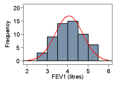
We will estimate the reference interval for FEV1 in male medical students. We have 57 observations, mean 4.06 and standard deviation 0.67 litres. The observations appear to follow a distribution which is close to the Normal (Figure 1).
Figure 1. FEV of 57 male medical students and Normal curve
with same mean and standard deviation
 D
D
The reference interval is thus 4.06 – 2×0.67 = 2.7 to 4.06 + 2×0.0.67 = 5.4 litres. From Table 1 we can see that in fact only one student (2%) is outside these limits, although the sample is rather small.
As the observations are assumed to be from a Normal distribution,
standard errors and confidence intervals for these
limits are easy to find.
Standard errors for 95% reference limits are approximately equal to
 .
Hence, provided Normal assumptions hold, we can find a
simple confidence interval for the limit.
For the FEV1 data, the standard error is
 .
Hence the 95% confidence intervals for these limits are
2.7 ± 1.96× 0.15 and 5.4 ± 1.96×0.15, i.e. from 2.4 to 3.0 and 5.1 to 5.7 litres.
The FEV data of Table 1 had a symmetrical distibution which made the estimation of the central 95% range using mean and standard deviation straightforward. Compare the serum triglyceride measurements of Table 2.
| 0.15 | 0.29 | 0.32 | 0.36 | 0.40 | 0.42 | 0.46 | 0.50 | 0.56 | 0.60 | 0.70 | 0.86 |
| 0.16 | 0.29 | 0.33 | 0.36 | 0.40 | 0.42 | 0.46 | 0.50 | 0.56 | 0.60 | 0.72 | 0.87 |
| 0.20 | 0.29 | 0.33 | 0.36 | 0.40 | 0.42 | 0.47 | 0.52 | 0.56 | 0.60 | 0.72 | 0.88 |
| 0.20 | 0.29 | 0.33 | 0.36 | 0.40 | 0.44 | 0.47 | 0.52 | 0.56 | 0.61 | 0.74 | 0.88 |
| 0.20 | 0.29 | 0.33 | 0.36 | 0.40 | 0.44 | 0.47 | 0.52 | 0.56 | 0.62 | 0.75 | 0.95 |
| 0.20 | 0.29 | 0.33 | 0.36 | 0.40 | 0.44 | 0.47 | 0.52 | 0.56 | 0.62 | 0.75 | 0.96 |
| 0.21 | 0.30 | 0.33 | 0.36 | 0.40 | 0.44 | 0.47 | 0.52 | 0.56 | 0.63 | 0.76 | 0.96 |
| 0.22 | 0.30 | 0.33 | 0.36 | 0.40 | 0.44 | 0.48 | 0.52 | 0.56 | 0.64 | 0.76 | 0.99 |
| 0.24 | 0.30 | 0.33 | 0.37 | 0.40 | 0.44 | 0.48 | 0.52 | 0.56 | 0.64 | 0.78 | 1.01 |
| 0.25 | 0.30 | 0.34 | 0.37 | 0.40 | 0.44 | 0.48 | 0.53 | 0.57 | 0.64 | 0.78 | 1.02 |
| 0.26 | 0.30 | 0.34 | 0.37 | 0.40 | 0.44 | 0.48 | 0.54 | 0.57 | 0.64 | 0.78 | 1.02 |
| 0.26 | 0.30 | 0.34 | 0.37 | 0.40 | 0.44 | 0.48 | 0.54 | 0.58 | 0.64 | 0.78 | 1.04 |
| 0.26 | 0.30 | 0.34 | 0.38 | 0.40 | 0.45 | 0.48 | 0.54 | 0.58 | 0.65 | 0.78 | 1.08 |
| 0.27 | 0.30 | 0.34 | 0.38 | 0.40 | 0.45 | 0.48 | 0.54 | 0.58 | 0.66 | 0.78 | 1.11 |
| 0.27 | 0.30 | 0.34 | 0.38 | 0.41 | 0.45 | 0.48 | 0.54 | 0.58 | 0.66 | 0.80 | 1.20 |
| 0.27 | 0.31 | 0.34 | 0.38 | 0.41 | 0.45 | 0.48 | 0.54 | 0.59 | 0.66 | 0.80 | 1.28 |
| 0.28 | 0.31 | 0.34 | 0.38 | 0.41 | 0.45 | 0.48 | 0.55 | 0.59 | 0.66 | 0.82 | 1.64 |
| 0.28 | 0.32 | 0.35 | 0.39 | 0.41 | 0.45 | 0.48 | 0.55 | 0.59 | 0.66 | 0.82 | 1.66 |
| 0.28 | 0.32 | 0.35 | 0.39 | 0.41 | 0.46 | 0.48 | 0.55 | 0.59 | 0.67 | 0.82 | |
| 0.28 | 0.32 | 0.35 | 0.39 | 0.41 | 0.46 | 0.49 | 0.55 | 0.60 | 0.67 | 0.82 | |
| 0.28 | 0.32 | 0.35 | 0.39 | 0.41 | 0.46 | 0.49 | 0.55 | 0.60 | 0.68 | 0.83 | |
| 0.28 | 0.32 | 0.35 | 0.39 | 0.42 | 0.46 | 0.49 | 0.55 | 0.60 | 0.70 | 0.84 | |
| 0.28 | 0.32 | 0.35 | 0.40 | 0.42 | 0.46 | 0.50 | 0.55 | 0.60 | 0.70 | 0.84 | |
| 0.28 | 0.32 | 0.36 | 0.40 | 0.42 | 0.46 | 0.50 | 0.55 | 0.60 | 0.70 | 0.84 |
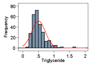
As Figure 2 shows, the data are highly skewed, and we cannot use the Normal method directly.
Figure 2. Serum triglyceride measurements in cord blood
from 282 babies and Normal curve with same mean and standard deviation
 D
D
If we did, the lower limit would be 0.07, well below any of the observations, and the upper limit would be 0.94, greater than which are 5% of the observations. It is possible for such data to give a negative lower limit.
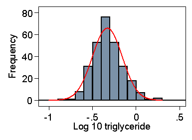
Figure 3 shows the log10 transformed data, which give a breathtakingly symmetrical distribution.
Figure 3. Log10 transformed serum triglyceride measurements
in cord blood from 282 babies and Normal curve with same
mean and standard deviation
 D
D
The mean and standard deviation are –0.331 and 0.171. The lower limit in the log transformed data is –0.331 – 2×0.171 = –0.673. If we antilog this, we get a triglyceride level equal to 0.21. 2.1% of observations are below this. The upper limit is –0.331 + 2×0.171 = 0.011. If we antilog this, we get a triglyceride level equal to 1.02, above which are 2.5% of observations. As Figure 3 shows, the fit of the log transformed data to a Normal distribution is excellent.
For the standard error of the reference limit we have
 .
The 95% confidence intervals are thus –0.673 ± 1.96×0.0176
and 0.011 ± 1.96×0.0176, i.e. –0.707 to –0.639 and
–0.023 to 0.045.
Transforming back to the linear scale, we get 0.20 to 0.23 and
0.95 to 1.11, found by taking the antilogs.
These confidence limits can be transformed back to the
original scale because no subtraction of means has taken place.
Because of the obviously unsatisfactory nature of the Normal method for some data, some authors have advocated the estimation of the centiles directly, without any distributional assumptions. This is an attractive idea. We want to know the point below which 2.5% of values will fall. Let us simply rank the observations and find the point below which 2.5% of the observations fall.
For the 282 triglycerides, the 2.5 and 97.5 centiles are found as follows. For the 2.5 centile, we find the observation whose rank is 0.025×(282 + 1) = 7.08. The required quantile will be between the 7th and 8th observations. The 7th is 0.21, the 8th is 0.22 so the 2.5 centile would be estimated by 0.21 + (0.22 – 0.21)×(7.08 – 7) = 0.21. Similarly the 97.5 centile is 1.04.
This approach gives an unbiassed estimate whatever the distribution. The log transformed triglyceride would give exactly the same results. Note that the Normal theory limits from the log transformed data are very similar.
We now look at the confidence interval. This is estimated by a direct method which tells us which rank the observations at the lower and upper confidence limits will be (see Bland 2000 §8.9, §15.5). For the triglyceride data, for the lower limit of the reference range the 95% confidence interval will be from the 2nd to the 13th observations. The second observation is 0.16 and the 13th is 0.26, so the 95% confidence interval for the lower reference limit is 0.16 to 0.26. The corresponding calculation for the 97.5 centile gives the 270th to the 281st observation, giving a 95% confidence interval for the upper reference limit of 0.96 to 1.64.
These are wider confidence intervals than those found by the Normal method, those for the long tail particularly so. This method of estimating centiles in long tails is relatively imprecise.
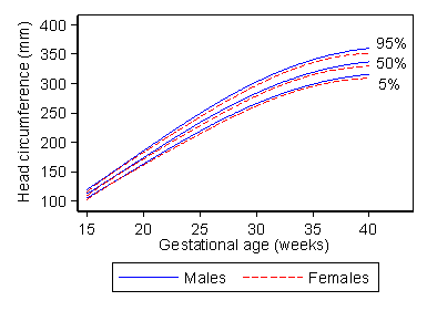
Centile charts show the reference range for different values of some other variable, usually age. For example, Figure 4 shows a 90% reference range for fetal head circumference.
Figure 4. Centile chart of fetal head circumference by
gestational age (Schwarzler et al., 2004)
 D
D
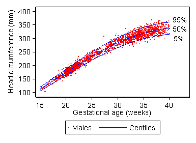
This enables us to see at the glance the range for fetuses of any gestational age. Like any reference range, the centile chart is estimated from data on an apparently normal set of subjects. The data used to produce the chart for males in Figure 4 are shown in Figure 5.
Figure 5. Data used to estimate the centile chart for males shown in
Figure 4
 D
D
In this case, it was important to exclude any extra measurements on fetuses made because there was concern about the development of the pregnancy, as these would produce a bias in the estimate.
Several different methods have been used to generate centile charts, but the best is due to Altman (1993). First we carry out regression with head circumference as the outcome (or dependent) variable and gestational age as the predictor (explanatory or independent) variable. We use a regression method which enables us to fit curves rather than straight lines. This enables us to estimate the mean head circumference for any gestational age. The problem is that the standard deviation can vary with gestational age, too. It clearly does so in Figure 5. We can estimate the standard deviation from the residuals, the differences between the observed values and those predicted by the regression equation.
Altman (1993) showed that, provided the residuals for any given gestational
age followed a Normal distribution, the absolute value
of the residual, without the + or – sign, can be used to estimate
the standard deviation.
We do regression with the absolute residual as the outcome variable
and gestational age as the predictor.
The standard deviation is given by the predicted absolute residual multiplied by
 .
We now have equations to predict the mean and the standard deviation
from the gestational age and we can use these to calculate the
centiles as we did for a simple reference range.
Altman DG. (1993) Construction of age-related reference centiles using absolute residuals. Stat Med 12, 917-924.
Bland M. (2000) An Introduction to Medical Statistics, 3rd Edition. Oxford University Press, Oxford.
Schwarzler P, Bland JM, Holden D, Campbell S, Ville Y. (2004) Sex-specific antenatal reference growth charts for uncomplicated singleton pregnancies at 15-40 weeks of gestation. Ultrasound in Obstetrics & Gynaecology 23, 23-29.
To Measurement in Health and Disease index.
To Martin Bland's M.Sc. index.
This page maintained by Martin Bland.
Last updated: 7 May, 2008.