2.6. Particle in a box with finite-potential walls

2.6.1. Authors

The Jupyter notebook is provided for the introductory Quantum Physics course at the University of York.

**These Jupyter notebooks are based on the excellent work by the following authors:

• Vinícius Wilian D. Cruzeiro. E-mail: vwcruzeiro@ufl.edu

• Xiang Gao. E-mail: qasdfgtyuiop@ufl.edu

• Valeria D. Kleiman. E-mail: kleiman@ufl.edu Department of Chemistry, Physical Chemistry Division, University of Florida**

Cite: J. Chem. Educ. 2019, 96, 8, 1663–1670, Publication Date:July 11, 2019. https://doi.org/10.1021/acs.jchemed.9b00195

Consider the case the situation of electrons in a metal. We saw when looking at the Photoelectric effect that a reasonable approximation of the potential that confines the electrons within the metal had a finite depth. This is the potential we will now consider and it is be far the most challenging problem you have met so far. Figure 2.3.1 shows a schematic representation of the finite square well. Unlike the infinite square well the finite potential well rises to a finite value of $V_0$ eV at $x=-L/2$ and $x=+L/2$.

2.6.2. The Schrödinger equation

$\begin{array}{ccc}\text{Inside the box}& \text{vs}& \text{Outside the box}\\ \frac{d^2\psi (x)}{d{x}^2}=-\frac{2mE}{{\hslash }^2}\psi (x)=-k^2\psi (x)& & \frac{d^2\psi (x)}{d{x}^2}=-\frac{2m(E-V_o)}{{\hslash }^2}\psi (x)\\ \text{Solutions have the general form of }\psi (x)=e^{\pm ikx}& & \text{If }E>V_o\text{, the particle is unbounded and}\\ \text{Therefore:}& & \text{the particle moves freely above the walls}\\ \psi (x)=q_1\cos (kx)+q_2\sin (kx)& & \text{If }E<V_o\text{, the particle is bounded and}\\ & & \text{within the walls}\end{array}$

For $E<V_o$, it is really interesting to look at what happens outside the walls.

When $E<V_o$, the Schrödinger equation becomes

$$\frac{{\partial }^2\psi (x)}{\partial x^2}={\beta }^2\cdot \psi (x)$$

since ${\beta }^2=\frac{2m(V_o-E)}{{\hslash }^2}>0$. The solutions to this equation have the general form of

$$\psi (x)=e^{\pm \beta x}.$$

Note that the exponential function doesn’t require an imaginary component, thus it is not oscillatory.

Before we move on, here are some questions to consider:

• Q1: Can you test if this is a solution to the differential equation?

• Q2 Can you write the general solution for a particle outside the box.

• Q3: What is the value of $\beta$?

• Q4: Given that $\psi (x)$ must be finite, how would this constrain the solutions for $x\to -\mathrm{\infty }$?

• Q5: Given that $\psi (x)$ must be finite, how would this constrain the solutions for $x\to \mathrm{\infty }$?

From the general solutions, and applying those constrains, we can consider three distinct regions.
In each region the wavefunction for $E<V_o$ will be:

$$\begin{array}{r}\begin{array}{llcl}I:& V(x)=Vo& x\le -\frac{L}{2}& {\psi }_I=A{e}^{\beta x}\\ II:& V(x)=0& -\frac{L}{2}\le x\le \frac{L}{2}& {\psi }_{II}=B\cos (kx)+C\sin (kx)\\ III:& V(x)=Vo& x\ge \frac{L}{2}& {\psi }_{III}=D{e}^{-\beta x}\end{array}\end{array}$$

where:

$${\alpha }_o=\frac{\sqrt{2m(V_o-E)}}{\hslash }k=\frac{\sqrt{2mE}}{\hslash }$$

Why do we check for continuity?

${\psi }^{{}^{\prime }}$ needs to be continuous to guarantee the existence of ${\psi }^{{}^{″}}$, whose existence is required from the first postulate. $\frac{d^2}{d{x}^2}$ is a component of the kinetic energy operator. If the wavefucntion doesn’t have a well-defined second derivative, then the kinetic energy would be undefined, which is not possible.

The wavefunction must obey the following boundary conditions:

${\psi }_I(-\frac{L}{2})={\psi }_{II}(-\frac{L}{2})$ and ${\psi }_{II}\left(\frac{L}{2}\right)={\psi }_{III}\left(\frac{L}{2}\right)$

${\psi }_I^{{}^{\prime }}(-\frac{L}{2})={\psi }_{II}^{{}^{\prime }}(-\frac{L}{2})$ and ${\psi }_{II}^{{}^{\prime }}\left(\frac{L}{2}\right)={\psi }_{III}^{{}^{\prime }}\left(\frac{L}{2}\right)$

where the symbol ${}^{\prime }$ corresponds to the first derivative with respect to $x$ (${\psi }^{{}^{\prime }}=\frac{d\psi }{dx}$)

It can be shown that when the potential is even ($V(-x)=V(x)$), the wavefunctions can be either even $[\psi (-x)=\psi (x)]$ or odd $[\psi (-x)=-\psi (x)]$.
On the way the potential is written, we are considering that the particle is in a finite box with an even potential. Thus, even and odd solutions of the wavefucntion can be found independently:

Even solutions:

$$\begin{array}{r}\begin{array}{ll}\text{For }x\le -\frac{L}{2}:& {\psi }_I(x)=D{e}^{\beta x}\\ \text{For }-\frac{L}{2}\le x\le \frac{L}{2}:& {\psi }_{II}(x)=B\cos (kx)\\ \text{For }x\ge \frac{L}{2}:& {\psi }_{III}(x)=D{e}^{-\beta x}\end{array}\end{array}$$

After imposing the boundary conditions we reach the following relation:

$$\begin{array}{}\text{(2)}& {\alpha }_o=k\tan \left(k\frac{L}{2}\right)\Rightarrow \sqrt{V_o-E}=\sqrt{E}\tan \left(\frac{L\sqrt{2mE}}{2\hslash }\right)\end{array}$$

Odd solutions:

$$\begin{array}{r}\begin{array}{ll}\text{For }x\le -\frac{L}{2}:& {\psi }_I(x)=-D{e}^{\beta x}\\ \text{For }-\frac{L}{2}\le x\le \frac{L}{2}:& {\psi }_{II}(x)=C\sin (kx)\\ \text{For }x\ge \frac{L}{2}:& {\psi }_{III}(x)=D{e}^{-\beta x}\end{array}\end{array}$$

After imposing the boundary conditions we reach the following relation:

$$\begin{array}{}\text{(3)}& {\alpha }_o=-\frac{k}{\tan \left(k\frac{L}{2}\right)}\Rightarrow \sqrt{V_o-E}=-\frac{\sqrt{E}}{\tan \left(\frac{L\sqrt{2mE}}{2\hslash }\right)}\end{array}$$

The actual solutions will be those corresponding to energies that obey equations 2 and 3. Once we find the allowed energies, we can go back and obtain the wavefunctions with the proper coefficients.

2.6.3. Finding the allowed Energies graphically

Unfortunately, we cannot find the allowed energies analytically. Instead we can do it graphically (first) or numerically (later). That is: we can graph the left and right hand side equations 2 and 3 and look for the intersection points. Those will correspond to the allowed energy values.

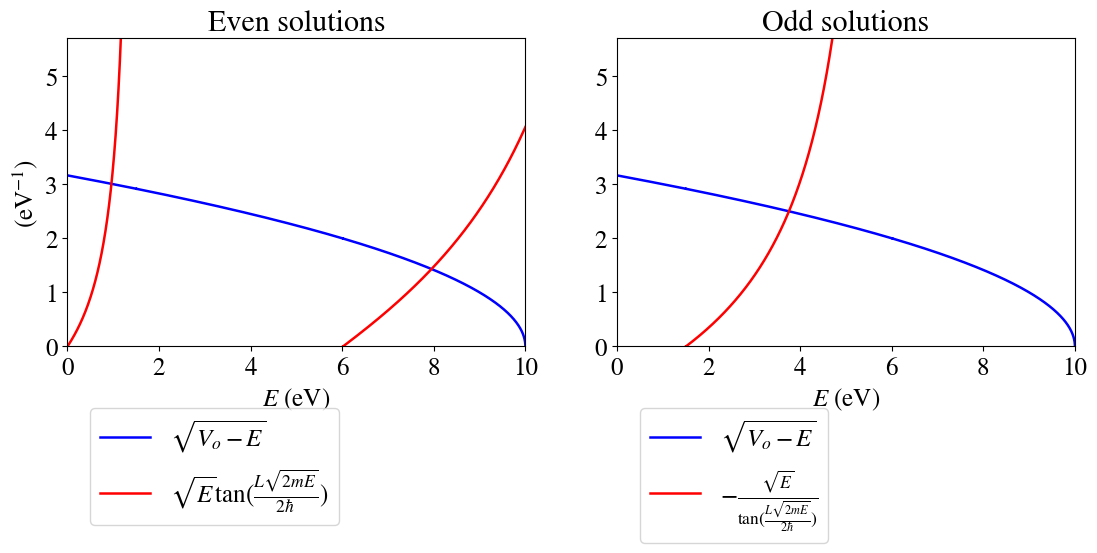
The allowed values would then be the values of $E$ in which the two curves cross. Here are some question to think about:

• Q1: How many bound states are possible?

• Q2: How many bound states are even and how many are odd?

• Q3: Is the ground state described by an even or an odd wavefunction?

• Q4: Can you read accuretely the allowed values of energy from these graphs?

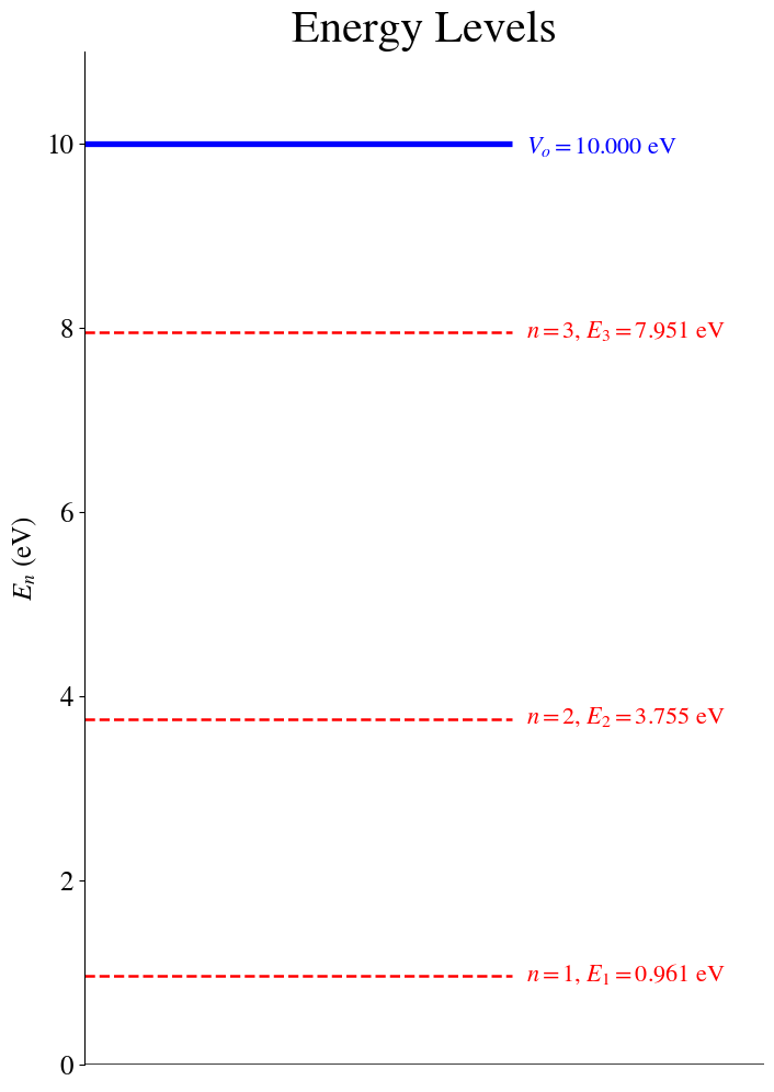
The allowed values of $E$ can be found by numerically, yielding:

The allowed bounded energies are:
  State #  1 (Even wavefunction):    0.9610 eV,   1.53974e-19 J

  State #  2  (Odd wavefunction):    3.7553 eV,   6.01664e-19 J

  State #  3 (Even wavefunction):    7.9505 eV,   1.27381e-18 J

THERE ARE   3 POSSIBLE BOUNDED ENERGIES

We can now plot these energy values as a diagram. Plotting an Energy Diagram helps us to see the energy separation between the states.

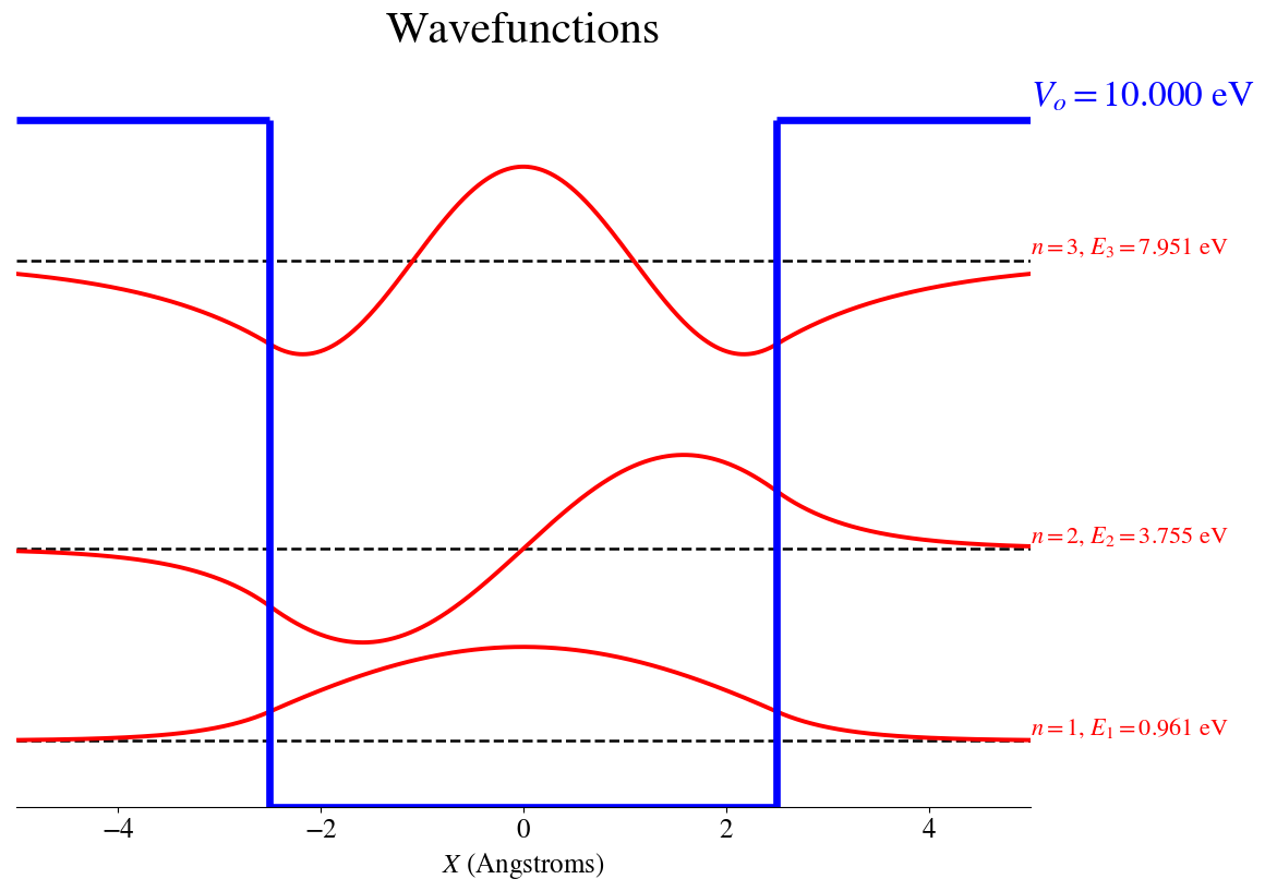
We can plug the values of $E$ back into the wavefunction expressions and plot the wavefunctions together with their corresponding probability densities.

The bound wavefunctions are:

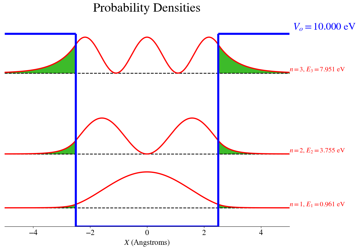
The bound Probability Densities are shown below 
with the areas shaded in green showing the regions where the particle can tunnel outside the box

If we compare these results with those of a particle in a box of same size but with infinite potential, we conclude that in the finite box, the levels are shifted to lower energies. More strikingly is the observation that the wavefunctions and the probability densities have non-zero values outside the box limits.

Classically, the particle cannot be found outside the box because the available energy is lower than the potential wall ($E<V_o$). However, for the particle in the finite box the wavefunction is nonzero outside the box, which means that there is a possibility of finding the particle outside the box. This is a pure quantum effect called the tunneling effect.

The tunneling probability correspond to the area outside the box that has non-zero values of probability density. In the graphicaly representation, those areas are shaded in green. The integration of those areas provide the probability that the particle will tunnel outside the classically allowed region.

$$\frac{{\int }_{-\mathrm{\infty }}^{\frac{-L}{2}}|\psi (x){|}^{2}dx+{\int }_{\frac{L}{2}}^{+\mathrm{\infty }}|\psi (x){|}^{2}dx}{{\int }_{-\mathrm{\infty }}^{+\mathrm{\infty }}|\psi (x){|}^{2}dx}$$

where the denominator is 1 for a normalized wavefunction.

This integral can be solved analytically (for the even and for the odd solutions). The tunneling probability for each state is:

The tunneling probabilities are:
  State #  1 tunneling probability =  1.98%
  State #  2 tunneling probability =  8.94%
  State #  3 tunneling probability = 28.06%

These evaluation and graphical representations show that the tunneling probability increases as the energy of the particle increases. This behavior is expected because, the higher the energy is, the lower the difference $V_o-E$ is, thus it becomes easier for the tunneling to happen. In other words, the closer the state is to the top of the potential barrier, the easier it is to spread outside.

Try evaluating these tunneling probabilities for different heights of the walls (different $V_o$ values). Do you expect the number of bound states to increase or decrease as $V_o$ increases?