RSS Statistics in Sports Section’s Olympic prediction competition 2024
0.1 Abstract
In this report we analyze and discuss the problem of predicting the Olympics medals table. The work presented here is informed by the ideas and findings of entrants to a Royal Statistical Society prediction competition, who competed to predict the medals table for the 2024 Olympic Games in Paris.
The entrants, who shared their predictions and methods, were: Jason West, Lexie Bonas, Alec Erskine, Joe Penn, Matt Penn, Fernando Zepeda, John Souza, John Edwards, Christopher Wharton, Ian Simpson, Orla Simpson, Tom Haynes, Mohamed Hammeda, Anik Saha, Amanda, John Fraser, Kaito Goto, Harry Snart and Chris Oates.
The competition entrants were given only a couple of weeks’ notice of the deadline and, in practice, few of them could devote more than a few hours to their submissions. In this way the competition acted as a case study in the utility of statistical ideas and software in the context of low computation- and time-budgets for model building and checking.
1 Introduction
1.1 Problem specification
In June 2024 the Statistics in Sport section of the Royal Statistical Society launched its annual prediction competition which, for this year, asked entrants to predict the medals table for the Summer Olympics held in Paris. Entrants were asked to rank 206 National Olympic Committees (NOCs) in terms of the number of gold medals they were expected to win. The metric chosen for scoring predictions is known as Kendall’s tau, a statistic that measures the correlation between the signs of the differences in a predicted ranking and a target ranking. More concretely, we write \[ \begin{align} \tau(\hat R,R) =& \frac{2}{n(n-1)} \sum_{i<j}\text{sign}(\hat R_i-\hat R_j)\text{sign}(R_i-R_j)\\ =& \frac{\text{number of concordant pairs}-\text{number of discordant pairs}}{\text{number of pairs}} \end{align} \tag{1}\] where \(\hat R_i\) denotes a predicted numerical rank for NOC \(i\) (e.g. if a forecaster predicted country \(i\) to be second from the top in the medals table they would set \(\hat R_i=2\)) and \(R_i\) denotes the true rank for country \(i\). It can be shown that \(\tau\) can also be formulated as a scaled difference between the number of pairs of NOCs that a forecaster puts in the correct order and the number they put in the wrong order. In the statistical literature the terms ‘concordant’ and ‘discordant’, respectively, are often used to describe these pairs.
Kendall’s tau is invariant to strictly increasing transformations of either of its arguments, meaning that only the ordering of the forecasted and realized rankings matter. As a consequence forecasters were free to specify non-integer ranks and negative ranks - anything that could be evaluated using Equation 1.
The \(\text{sign}\) function used here returns value one when its argument is positive, minus one when its argument is negative and zero when its argument is zero. This means that when a pair of NOCs are tied, either in the predicted or target ranking, then the pair does not contribute to the score. For the purposes of this competition the true final ranking was determined by the number of gold medals won by each country. Silver medals were used only to break ties between countries with equal numbers of gold medals. Bronze medals were used to break ties between countries after silver medals were accounted for. Countries still tied after accounting for bronze medals remained tied.
1.2 The relevance of ranking
The problem of ranking is central to statistical theory. Indeed, the need to rank preferences for actions with uncertain outcomes (i.e. gambles) is what motivates and informs the construction of subjectivist formalizations of probability from which Bayesian statistics (see the introductory chapters of Savage (1972)) and Game theory (via the Von Neumann–Morgenstern utility theorem of Von Neumann and Morgenstern (1947)) are derived. Ranking problems are also of considerable practical concern, particularly in the context of ‘recommender systems’ that provide ordered lists of recommendations for websites to visit or films to watch. In these ways, tackling ranking problems in practice has a track record for motivating progress in statistical theory and computation. It is our intention for the observations that we have made during the prediction competition to help the reader evaluate the utility of existing methods and to encourage the reader to produce their own.
2 Exploratory data analysis
In this section we make use primarily of a data set provided by Petro via the website Kaggle.com, which hosts a large number of prediction and analysis competitions. This well-curated data set records the results of all summer and winter Olympic events since 1896, collected together in the form of a data frame with approximately 163k rows and 15 columns.
2.1 Distribution of medal counts
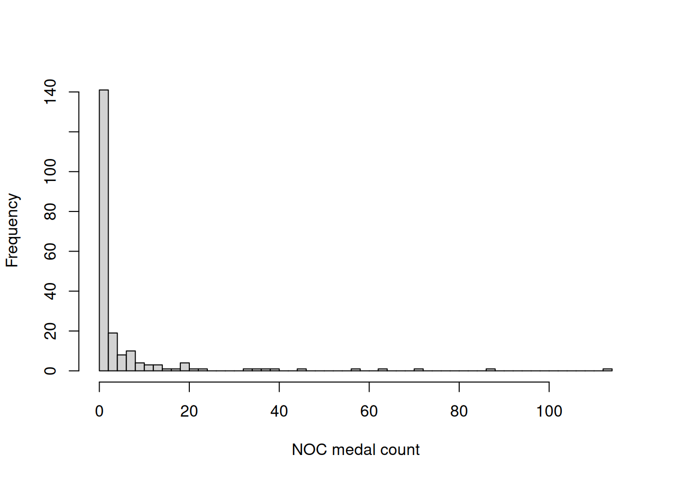
In Figure 1 we provide a histogram of the medal counts (adding gold, silver and bronze) for all NOCs competing at the 2020 Summer Olympics in Tokyo. It is clear that the majority of NOCs come home with very few, if any, medals while a small number come home with many. We can see this more clearly in Table 1, which tells us that 113 of 206 NOCs (\(\approx 55\%\)) received no medals in 2020, while China and the USA are far out in the tail of this distribution with 88 and 113 medals respectively.
The presence of a large number of NOCs tied at joint-last place with no medals and the absence of a weighting privileging NOCs with high medal counts has some interesting implications for our competition. It means, for instance, that in 2020 no forecaster could have achieved a Kendall’s tau score of more than \(\left(\binom{206}{2}-\binom{113}{2}\right)/\binom{206}{2} \approx 0.7\) because every summand in Equation 1 corresponding to a pair of NOCs with no medals evaluates to zero. It also means that a single medal being won by an NOC immediately puts them ahead of a large number of competitors tied at zero. In practice this rewarded forecasters for identifying NOCs with small total medal counts but high chances of winning a specific event for which they have a exceptional athlete.
Despite the large number of observed ties it is generally not a good idea to predict ties. This becomes apparent after noticing that the expected contribution to a forecaster’s score from a prediction that ranks NOC \(i\) ahead of NOC \(j\) is \(\propto P(R_i<R_j)-P(R_j<R_i)\). So even if the forecaster believes that \(R_i < R_j\) is only a tiny bit more probable than \(R_i > R_j\), the expected reward from specifying \(\hat R_i < \hat R_j\) is greater than specifying \(\hat R_i = \hat R_j\), which will lead to a zero contribution to the score. This remains the case even when \(P(R_i=R_j) \gg P(R_i \neq R_j)\). However, predicting ties could be justified on the basis that it reduces the variance of a forecaster’s score so that, for example, a forecaster who is confident in their ranking of the top 10 NOCs but unsure of the remaining 196 could protect themselves from ‘noise’ by forecasting these 196 to take joint last position.

| Medal count | 0 | 1 | 2 | 3 | 4 | 5 | 6 | 7 | 8 | 9 | 10 | 11 | 12 | 13 | 14 | 15 | 17 | 19 | 20 | 21 | 24 | 33 | 36 | 37 | 40 | 46 | 58 | 64 | 71 | 88 | 113 |
| Freq. | 113 | 17 | 11 | 6 | 13 | 5 | 3 | 6 | 4 | 3 | 1 | 2 | 1 | 2 | 1 | 1 | 1 | 1 | 3 | 1 | 1 | 1 | 1 | 1 | 1 | 1 | 1 | 1 | 1 | 1 | 1 |
2.2 Disaggregation by year
Next, we take a look at the variation in gold medal counts over time, focusing on the most recent games and NOCs with the highest medal counts. For now we consider only the games after the 1980 Moscow Olympics, which were notable for a boycott led by the USA. We note that a similar boycott led by the USSR affected the 1984 Los Angeles Olympics, but appears to have had a smaller effect on the medals table. The counts are presented in Table 2, where early figures for Russia and Germany are filled with NAs because they participated via different, and now defunct, NOCs. The totals on the bottom row of the table refer to the total number of gold medals awarded that year to all NOCs, not just to the subset corresponding to the rows above. These totals reflect a gradual increase in the number events.
The boycotts from the NOCs with the highest historical medal counts provide a warning against using too much of the Olympic data to fit our models. More specifically, time series of medal counts appearing to plummet suddenly to zero threaten to greatly skew estimated parameters in standard ARIMA-type models. It is easy to imagine that the boycotts are just one of many events that, while obvious at the time, are difficult to identify and rationalize as we look back through the data. The most straightforward strategy for dealing with this problem, and the one chosen by the majority of the competition entrants, was to fit models using only the most recent games (medal counts since 1996 or 2000 were common choices).
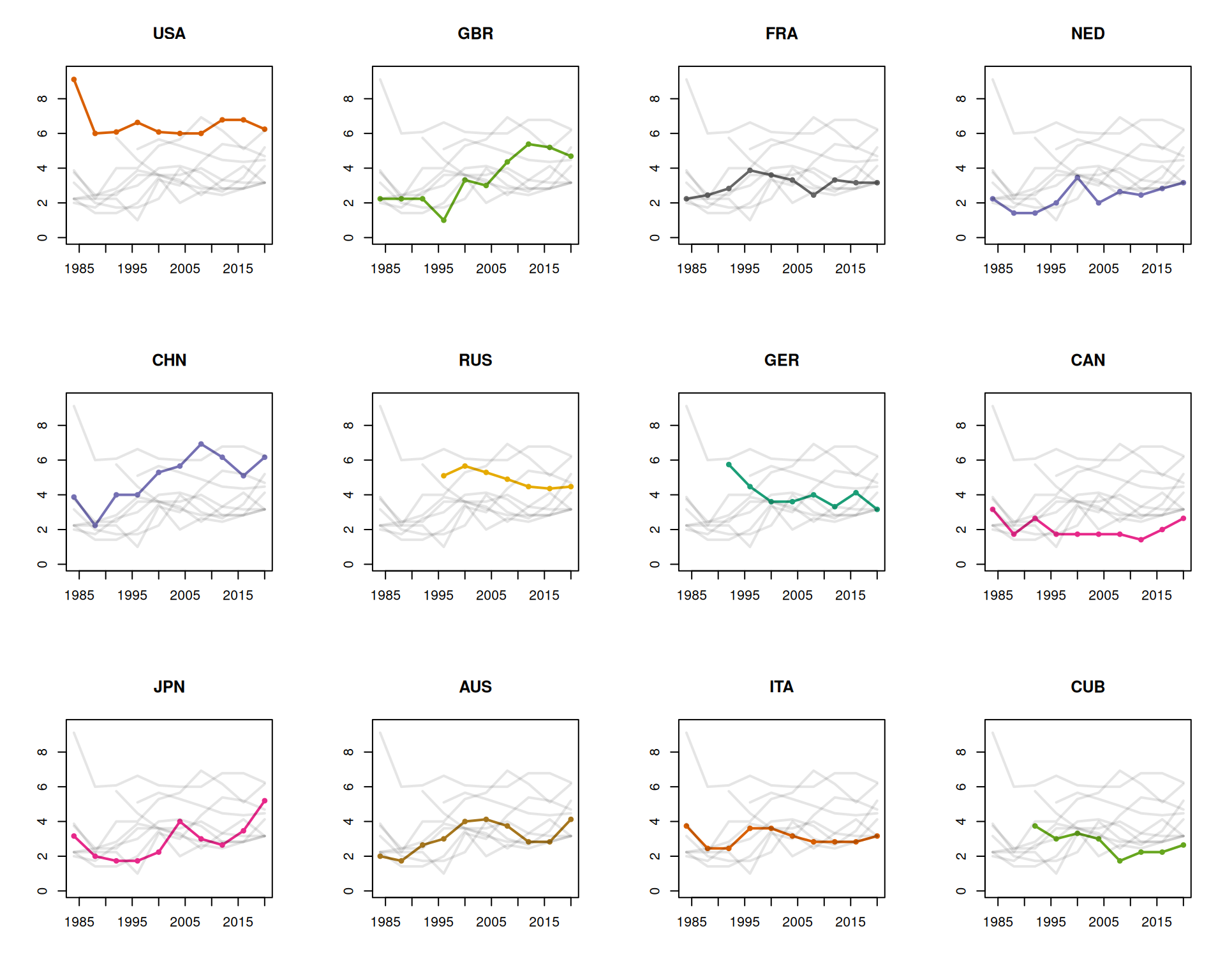
A visualization of the counts is provided in Figure 2 where we plot their square roots. This transformation helps us to differentiate between the lower counts and, in anticipation of later analyses, serves to stabilize their variance. For most of the NOCs here the gold medal counts appear to vary by only a small amount over the 40-year time window. China, Great Britain, Japan and Australia are characterized by upward trends.
| 1984 | 1988 | 1992 | 1996 | 2000 | 2004 | 2008 | 2012 | 2016 | 2020 | |
|---|---|---|---|---|---|---|---|---|---|---|
| USA | 83 | 36 | 37 | 44 | 37 | 36 | 36 | 46 | 46 | 39 |
| CHN | 15 | 5 | 16 | 16 | 28 | 32 | 48 | 38 | 26 | 38 |
| JPN | 10 | 4 | 3 | 3 | 5 | 16 | 9 | 7 | 12 | 27 |
| GBR | 5 | 5 | 5 | 1 | 11 | 9 | 19 | 29 | 27 | 22 |
| RUS | NA | NA | NA | 26 | 32 | 28 | 24 | 20 | 19 | 20 |
| AUS | 4 | 3 | 7 | 9 | 16 | 17 | 14 | 8 | 8 | 17 |
| FRA | 5 | 6 | 8 | 15 | 13 | 11 | 6 | 11 | 10 | 10 |
| GER | NA | NA | 33 | 20 | 13 | 13 | 16 | 11 | 17 | 10 |
| ITA | 14 | 6 | 6 | 13 | 13 | 10 | 8 | 8 | 8 | 10 |
| NED | 5 | 2 | 2 | 4 | 12 | 4 | 7 | 6 | 8 | 10 |
| CAN | 10 | 3 | 7 | 3 | 3 | 3 | 3 | 2 | 4 | 7 |
| CUB | NA | NA | 14 | 9 | 11 | 9 | 3 | 5 | 5 | 7 |
| totals | 226 | 149 | 260 | 271 | 300 | 301 | 301 | 301 | 307 | 339 |
2.3 Disaggregation by discipline
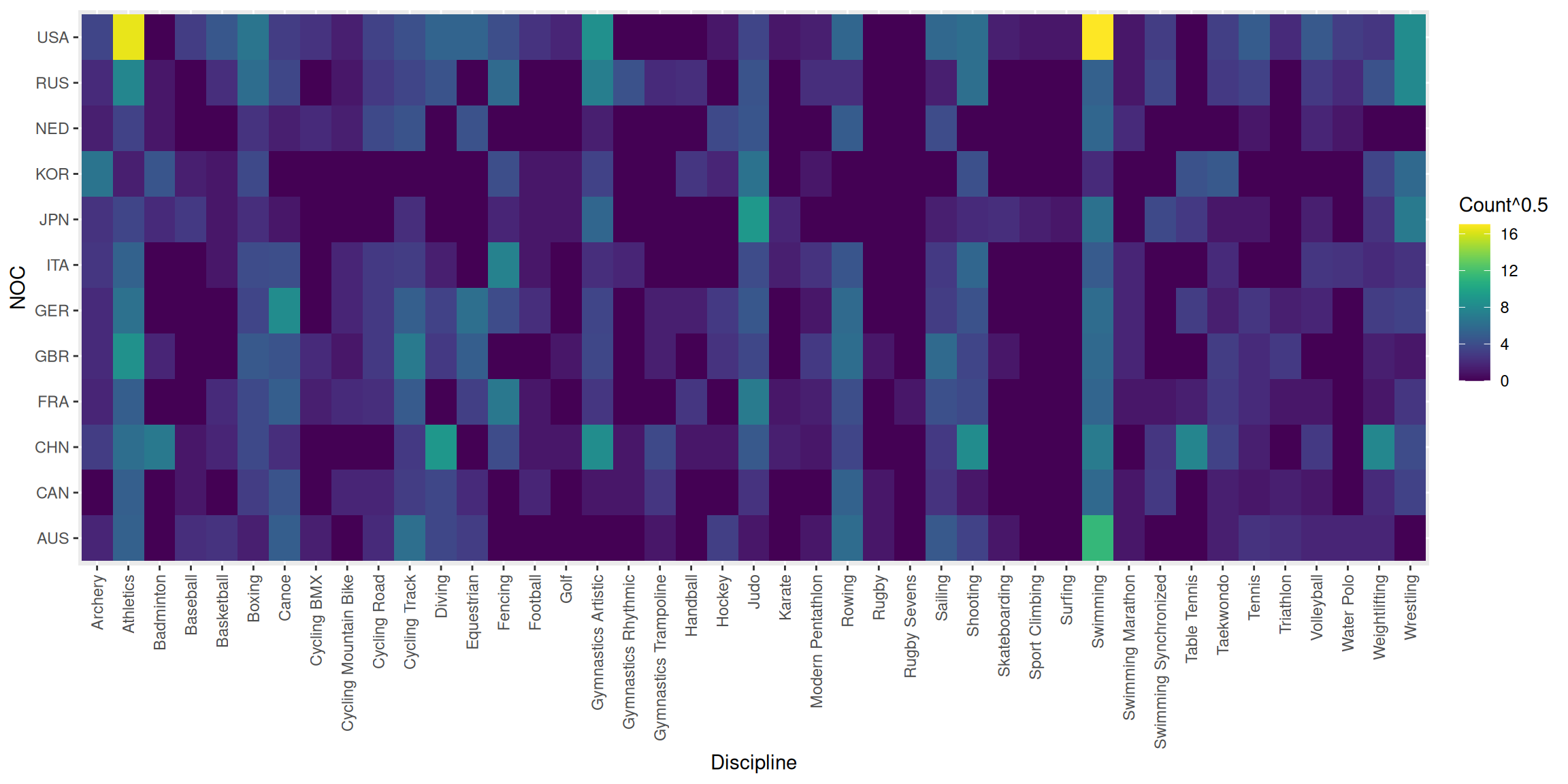
We now explore the similarities between NOCs in terms of the sporting disciplines they tend to win medals in and, analogously, the similarities between disciplines in terms of the countries that tend to win medals in them. Our starting point is Table 4, which contains the total gold medal counts for a subset of the most successful NOCs between 1984 and 2020. This data in plotted in the form a heatmap in Figure 4, in which we can see the large number of medals awarded for swimming and athletics and the dominance of the USA in these disciplines.
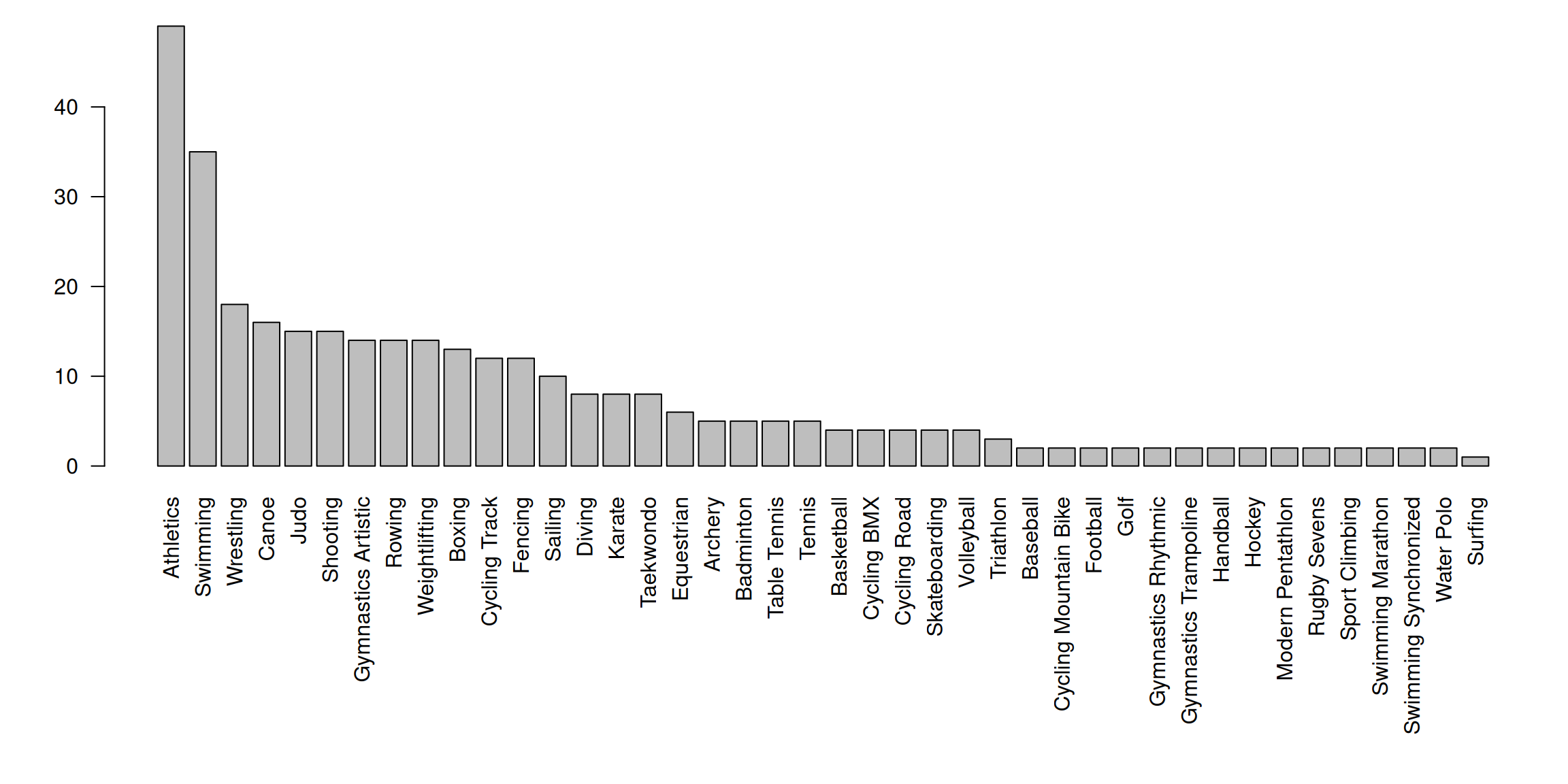
In Table 3 we present the counts for the total number of gold medals awarded for each of a set of disciplines at recent Summer Olympics. We see firstly that most medals are awarded for athletics and swimming, followed by combat sports: wrestling, judo and boxing. It is also interesting to look at the variability of these counts. Specifically, we draw attention to the introduction of Karate and Taekwondo part way through the period considered which each introduce an extra 8 gold medals. This reminds us that changes in an NOC’s medal count may be attributable to variation in their athletes and to the composition of the games themselves. A convenient way to at least partially address the changing medal counts for the disciplines when making forecasts is, for each year and NOC, to divide the medal count by the number available that year (plus a small constant to avoid zero-division) and multiplying by the number available in 2024. In this way we adjust the historical data in such a way that it more closely reflects the 2024 games.
| 1984 | 1988 | 1992 | 1996 | 2000 | 2004 | 2008 | 2012 | 2016 | 2020 | |
|---|---|---|---|---|---|---|---|---|---|---|
| Archery | 2 | 4 | 4 | 4 | 4 | 4 | 4 | 4 | 4 | 5 |
| Athletics | 41 | 26 | 43 | 44 | 45 | 46 | 47 | 46 | 47 | 49 |
| Badminton | 0 | 0 | 4 | 5 | 5 | 5 | 5 | 5 | 5 | 5 |
| Baseball | 0 | 0 | 1 | 2 | 2 | 2 | 2 | 0 | 0 | 2 |
| Basketball | 2 | 1 | 2 | 2 | 2 | 2 | 2 | 2 | 2 | 4 |
| Boxing | 12 | 9 | 12 | 12 | 12 | 11 | 11 | 13 | 13 | 13 |
| Canoe | 12 | 6 | 16 | 16 | 16 | 16 | 16 | 16 | 16 | 16 |
| Cycling BMX | 0 | 0 | 0 | 0 | 0 | 0 | 2 | 2 | 2 | 4 |
| Cycling Mountain Bike | 0 | 0 | 0 | 2 | 2 | 2 | 1 | 2 | 2 | 2 |
| Cycling Road | 3 | 1 | 3 | 4 | 4 | 4 | 4 | 4 | 4 | 4 |
| Cycling Track | 5 | 1 | 7 | 8 | 12 | 12 | 10 | 10 | 10 | 12 |
| Diving | 4 | 4 | 4 | 4 | 8 | 8 | 8 | 8 | 8 | 8 |
| Equestrian | 6 | 6 | 6 | 6 | 6 | 6 | 6 | 6 | 6 | 6 |
| Fencing | 8 | 7 | 8 | 10 | 10 | 10 | 10 | 10 | 10 | 12 |
| Football | 1 | 0 | 1 | 2 | 2 | 2 | 2 | 2 | 2 | 2 |
| Golf | 0 | 0 | 0 | 0 | 0 | 0 | 0 | 0 | 2 | 2 |
| Gymnastics Artistic | 18 | 6 | 16 | 14 | 14 | 14 | 14 | 14 | 14 | 14 |
| Gymnastics Rhythmic | 1 | 0 | 1 | 2 | 2 | 2 | 2 | 2 | 2 | 2 |
| Gymnastics Trampoline | 0 | 0 | 0 | 0 | 2 | 2 | 2 | 2 | 2 | 2 |
| Handball | 2 | 1 | 2 | 2 | 2 | 2 | 2 | 2 | 2 | 2 |
| Hockey | 2 | 2 | 2 | 2 | 2 | 2 | 2 | 2 | 2 | 2 |
| Judo | 8 | 7 | 14 | 14 | 14 | 14 | 14 | 14 | 14 | 15 |
| Karate | 0 | 0 | 0 | 0 | 0 | 0 | 0 | 0 | 0 | 8 |
| Modern Pentathlon | 2 | 2 | 2 | 1 | 2 | 2 | 2 | 2 | 2 | 2 |
| Rowing | 14 | 6 | 14 | 14 | 14 | 14 | 14 | 14 | 14 | 14 |
| Rugby | 0 | 0 | 0 | 0 | 0 | 0 | 0 | 0 | 2 | 0 |
| Rugby Sevens | 0 | 0 | 0 | 0 | 0 | 0 | 0 | 0 | 0 | 2 |
| Sailing | 7 | 7 | 10 | 10 | 11 | 11 | 11 | 10 | 10 | 10 |
| Shooting | 11 | 8 | 13 | 15 | 17 | 17 | 15 | 15 | 15 | 15 |
| Skateboarding | 0 | 0 | 0 | 0 | 0 | 0 | 0 | 0 | 0 | 4 |
| Sport Climbing | 0 | 0 | 0 | 0 | 0 | 0 | 0 | 0 | 0 | 2 |
| Surfing | 0 | 0 | 0 | 0 | 0 | 0 | 0 | 0 | 0 | 1 |
| Swimming | 30 | 18 | 31 | 32 | 33 | 32 | 32 | 32 | 33 | 35 |
| Swimming Marathon | 0 | 0 | 0 | 0 | 0 | 0 | 2 | 2 | 2 | 2 |
| Swimming Synchronized | 2 | 2 | 3 | 1 | 2 | 2 | 2 | 2 | 2 | 2 |
| Table Tennis | 0 | 4 | 4 | 4 | 4 | 4 | 4 | 4 | 4 | 5 |
| Taekwondo | 0 | 0 | 0 | 0 | 8 | 8 | 8 | 8 | 8 | 8 |
| Tennis | 0 | 4 | 4 | 4 | 4 | 4 | 4 | 5 | 5 | 5 |
| Triathlon | 0 | 0 | 0 | 0 | 2 | 2 | 2 | 2 | 2 | 3 |
| Volleyball | 2 | 1 | 2 | 4 | 4 | 4 | 4 | 4 | 4 | 4 |
| Water Polo | 1 | 1 | 1 | 1 | 2 | 2 | 2 | 2 | 2 | 2 |
| Weightlifting | 10 | 3 | 10 | 10 | 15 | 15 | 15 | 14 | 15 | 14 |
| Wrestling | 20 | 12 | 20 | 20 | 16 | 18 | 18 | 19 | 18 | 18 |
| Archery | Athletics | Badminton | Baseball | Basketball | Boxing | Canoe | Cycling BMX | Cycling Mountain Bike | Cycling Road | Cycling Track | Diving | Equestrian | Fencing | Football | Golf | Gymnastics Artistic | Gymnastics Rhythmic | Gymnastics Trampoline | Handball | Hockey | Judo | Karate | Modern Pentathlon | Rowing | Rugby | Rugby Sevens | Sailing | Shooting | Skateboarding | Sport Climbing | Surfing | Swimming | Swimming Marathon | Swimming Synchronized | Table Tennis | Taekwondo | Tennis | Triathlon | Volleyball | Water Polo | Weightlifting | Wrestling | |
|---|---|---|---|---|---|---|---|---|---|---|---|---|---|---|---|---|---|---|---|---|---|---|---|---|---|---|---|---|---|---|---|---|---|---|---|---|---|---|---|---|---|---|---|
| USA | 12 | 271 | 0 | 9 | 21 | 44 | 9 | 6 | 2 | 11 | 17 | 29 | 29 | 16 | 6 | 3 | 72 | 0 | 0 | 0 | 1 | 12 | 1 | 2 | 31 | 0 | 0 | 32 | 37 | 2 | 1 | 1 | 290 | 1 | 9 | 0 | 10 | 24 | 4 | 22 | 9 | 7 | 68 |
| CHN | 9 | 37 | 47 | 1 | 3 | 14 | 5 | 0 | 0 | 0 | 8 | 81 | 0 | 15 | 1 | 1 | 69 | 1 | 14 | 1 | 1 | 22 | 2 | 1 | 12 | 0 | 0 | 8 | 67 | 0 | 0 | 0 | 49 | 0 | 7 | 60 | 11 | 2 | 0 | 8 | 0 | 62 | 15 |
| RUS | 4 | 61 | 1 | 0 | 5 | 36 | 13 | 0 | 1 | 8 | 12 | 19 | 0 | 34 | 0 | 0 | 52 | 18 | 4 | 5 | 0 | 19 | 0 | 5 | 5 | 0 | 0 | 2 | 38 | 0 | 0 | 0 | 27 | 1 | 12 | 0 | 8 | 11 | 0 | 8 | 4 | 18 | 64 |
| GER | 4 | 39 | 0 | 0 | 0 | 12 | 67 | 0 | 3 | 8 | 26 | 11 | 38 | 15 | 5 | 0 | 12 | 0 | 2 | 2 | 8 | 21 | 0 | 1 | 34 | 0 | 0 | 9 | 18 | 0 | 0 | 0 | 35 | 3 | 0 | 9 | 2 | 7 | 2 | 3 | 0 | 9 | 11 |
| GBR | 4 | 73 | 3 | 0 | 0 | 22 | 19 | 4 | 1 | 8 | 48 | 8 | 25 | 0 | 0 | 1 | 13 | 0 | 2 | 0 | 6 | 13 | 0 | 8 | 36 | 1 | 0 | 34 | 12 | 1 | 0 | 0 | 33 | 3 | 0 | 0 | 9 | 4 | 8 | 0 | 0 | 2 | 1 |
| AUS | 3 | 27 | 0 | 5 | 6 | 2 | 25 | 2 | 0 | 4 | 38 | 13 | 9 | 0 | 0 | 0 | 0 | 0 | 1 | 0 | 10 | 1 | 0 | 1 | 35 | 1 | 0 | 22 | 11 | 1 | 0 | 0 | 129 | 1 | 0 | 0 | 2 | 6 | 5 | 3 | 3 | 3 | 0 |
| FRA | 3 | 25 | 0 | 0 | 4 | 14 | 25 | 2 | 4 | 5 | 23 | 0 | 10 | 46 | 1 | 0 | 7 | 0 | 0 | 7 | 0 | 49 | 1 | 2 | 16 | 0 | 1 | 17 | 14 | 0 | 0 | 0 | 30 | 1 | 1 | 2 | 8 | 4 | 1 | 1 | 0 | 1 | 7 |
| JPN | 6 | 12 | 4 | 8 | 1 | 5 | 1 | 0 | 0 | 0 | 5 | 0 | 0 | 3 | 1 | 1 | 31 | 0 | 0 | 0 | 0 | 83 | 3 | 0 | 0 | 0 | 0 | 2 | 4 | 5 | 2 | 1 | 40 | 0 | 14 | 8 | 1 | 1 | 0 | 2 | 0 | 6 | 48 |
| ITA | 7 | 28 | 0 | 0 | 1 | 15 | 16 | 0 | 3 | 8 | 9 | 2 | 0 | 56 | 1 | 0 | 5 | 3 | 0 | 0 | 0 | 15 | 2 | 6 | 20 | 0 | 0 | 8 | 31 | 0 | 0 | 0 | 23 | 3 | 0 | 0 | 4 | 0 | 0 | 7 | 6 | 4 | 6 |
| KOR | 43 | 2 | 20 | 2 | 1 | 14 | 0 | 0 | 0 | 0 | 0 | 0 | 0 | 16 | 1 | 1 | 11 | 0 | 0 | 7 | 3 | 41 | 0 | 1 | 0 | 0 | 0 | 0 | 17 | 0 | 0 | 0 | 4 | 0 | 0 | 18 | 22 | 0 | 0 | 0 | 0 | 12 | 33 |
| CAN | 0 | 26 | 0 | 1 | 0 | 9 | 19 | 0 | 3 | 3 | 9 | 13 | 4 | 0 | 3 | 0 | 1 | 1 | 7 | 0 | 0 | 6 | 0 | 0 | 28 | 1 | 0 | 6 | 1 | 0 | 0 | 0 | 33 | 1 | 8 | 0 | 2 | 1 | 2 | 1 | 0 | 4 | 11 |
| NED | 2 | 11 | 1 | 0 | 0 | 6 | 2 | 4 | 2 | 14 | 19 | 0 | 18 | 0 | 0 | 0 | 2 | 0 | 0 | 0 | 14 | 20 | 0 | 0 | 24 | 0 | 0 | 15 | 0 | 0 | 0 | 0 | 31 | 4 | 0 | 0 | 0 | 1 | 0 | 3 | 1 | 0 | 0 |
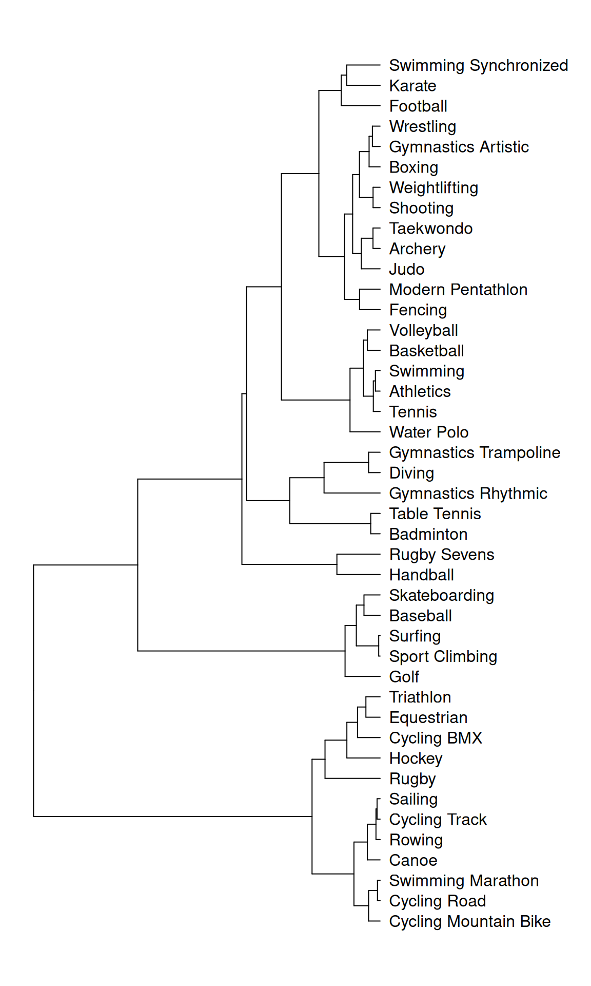
We proceed by treating each column of Table 4 as though it were an unnormalized probability distribution over NOCs and then computing a statistical distance between them. These distances are used as inputs for a hierarchical clustering algorithm whose output is plotted in Figure 5. Specifically, we use the Hellinger distance and the Ward cluster agglomeration method. It is interesting to see a cluster containing the ‘sitting-down’ sports, which tend to be associated with wealthier NOCs and include the equestrian events, rowing, sailing, canoe and cycling; and a small number of clusters containing most of the combat sports.
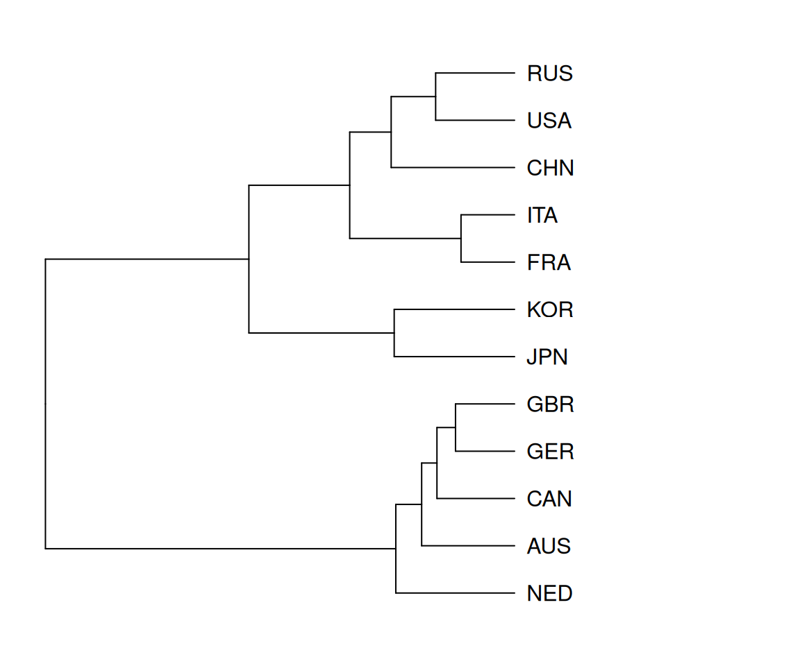
The same clustering procedure can be applied to the rows of Table 4, leading to Figure 6. It is tempting to interpret clusters here in terms of the NOC’s climates and cultures, which influence the events they invest in most heavily. The short tree distances between Italy and France, and Germany and Great Britain, for example, could be understood as resulting from cultural similarities. We also observe a relatively small distance between the USA and Russia, whose investments in similar events could be attributed to their historic soft-power competitions as rival global superpowers.
In both dendrogram plots the vertical displacement has no real significance. The horizontal positions at which clusters merge is indicative of their distance before merging so that, for example, table tennis and badminton are closer together than rugby sevens and handball. The idea motivating these exploratory analyses is that an NOC’s strength in a particular discipline might be inferred by its success in another. For example, there might be an NOC who gained medals in 2020 in surfing but not sport climbing; knowing the association between the two disciplines might increase our prediction for that country’s chances of winning a medal for sport climbing in 2024.
The dendrogram in Figure 5 provides us with a starting point for thinking about different levels of aggregation of medal data and, more specifically, about the level of aggregation at which we should be constructing models. Well established results from the time series literature, namely Granger and Morris (1976), tell us that additive sums of ARIMA processes lead to ARIMA processes whose dependence on the past gets longer. In this sense there is a trade-off between additively aggregating ARIMA processes and keeping down the number of lagged observations needed to predict future values. Conversely, disaggregating the series of medal counts ought to allow us to infer high-order ARIMA coefficients of the aggregated count even without a long series of observations. In this sense, the availability of the extra disaggregated data is comparable to the availability of a longer series of observed aggregated counts, which ought to improve our forecasts.
If we disaggregate too far, however, we may encounter the problem of having very many zero counts which poses difficulties for parameter estimation, at least for standard Poisson regression methods. An implication is that there is some intermediate level of aggregation that will help us predict the total medal counts most accurately.
We note that, intuitively, arguments in favour of disaggregating the medal counts and fitting different models to them would be supported if these sub-counts exhibited distinct dynamic behaviours. This could arise, for instance, if athletes in some disciplines (e.g. archery and shooting) had longer careers than others or if the infrastructure needed to participate in some disciplines (e.g. special training facilities) had a longer lifetime than others. Given these ideas, when predicting future medal counts, we may want to treat medals for events in which expertise is in some way more persistent over time differently from other medals.
2.4 The absence of Russian athletes
The 2024 Summer Olympics were notable for the absence of athletes from Russia. It is interesting to consider whether this allowed NOCs who have traditionally competed with Russia in certain disciplines to gain more medals than NOCs who concentrated mostly on disciplines with relatively little Russian involvement. Such a non-uniform redistribution of medals could be expected to have an effect on the final medals table ranking.
Forecasters using bookmakers odds, or their own sporting knowledge, and making predictions for the 2024 games at the level of individual events were able to implicitly account for the Russian absence. They allotted fractions of expected gold medals to participating NOCs in line with their track records for particular events. Forecasters working at the level of total medal counts, however, generally could not make equivalent adjustments. It could be said that they relied on the medals that would have been won by Russia being uniformly redistributed over the other NOCs so that their expected medal counts are inflated but their ordering remains the same. It is interesting, however, to see if a more sophisticated calculation would have been beneficial.
The non-uniform redistribution of medals alluded to above can be formalized in an equation like Equation 2, whose left-hand side is to be read as ‘the probability that NOC \(j\) wins a medal in 2024 given that Russia would have won it, had it been participating’. This probability is decomposed, via the law of marginal probability, according to the discipline the hypothetical medal is won in. The joint probabilities are then expressed as the product of conditional and marginal distributions. Finally, we assert that \(P(\text{NOC}_j \mid \text{disc}_i, \text{RUS})=P(\text{NOC}_j \mid \text{disc}_i)\), reflecting the idea that Russia’s absence frees up a medal in discipline \(i\) but Russia cannot transfer it directly to any other NOC. \[ \begin{align} P(\text{NOC}_j \mid \text{RUS}) =& \sum_i P(\text{NOC}_j, \text{disc}_i \mid \text{RUS}) \\ =& \sum_i P(\text{NOC}_j \mid \text{disc}_i, \text{RUS}) \ P(\text{disc}_i | \text{RUS}) \\ =& \sum_i P(\text{NOC}_j \mid \text{disc}_i) \ P(\text{disc}_i | \text{RUS}) \end{align} \tag{2}\] We can estimate the factors in the final line of Equation 2 from our data simply by computing the proportions of disciplines in which Russia has historically won medals (for \(P(\text{disc}_i | \text{RUS})\)) and the proportion of medals won by different NOCs (excluding Russia) in a particular discipline (for the \(P(\text{NOC}_j \mid \text{disc}_i)\)). A subset of the relevant data can be seen above in Figure 4. Now, if we proceed to forecast the 2024 Russian medal count without accounting for their non-participation we can perform a correction whereby this count is multiplied by \(P(\text{NOC}_j \mid \text{RUS})\) and added on to the counts for the other NOCs, before being set to zero. The values of \(P(\text{NOC}_j \mid \text{RUS})\) that we compute this way turn out to be largest for USA, China, Italy and Japan which is partly because these NOCs tend to win lots of medals anyway, i.e. their values for \(P(\text{NOC}_j \mid \text{disc}_i)\) tend to be large. Perhaps more importantly for predicting ranks, however, large values of \(P(\text{NOC}_j \mid \text{RUS})\) as a fraction of the NOCs’ average previous medal counts are computed for Israel, Kyrgyzstan, Bulgaria and Ukraine. Small increases to the medal counts for these NOCs could lead to large differences in their rankings.
Equation 2 is a nice example of a Bayesian counterfactual calculation, which are often causes of confusion because it seems as though we are simultaneously conditioning on an event and its complement - in this case Russia winning and not winning a particular medal. The story accompanying the calculation in our case, however, makes the calculation easier to intuit since we can imagine Russia winning a medal in a discipline, having to give it up and it then being competed for among the other NOCs.
3 Gathering additional data
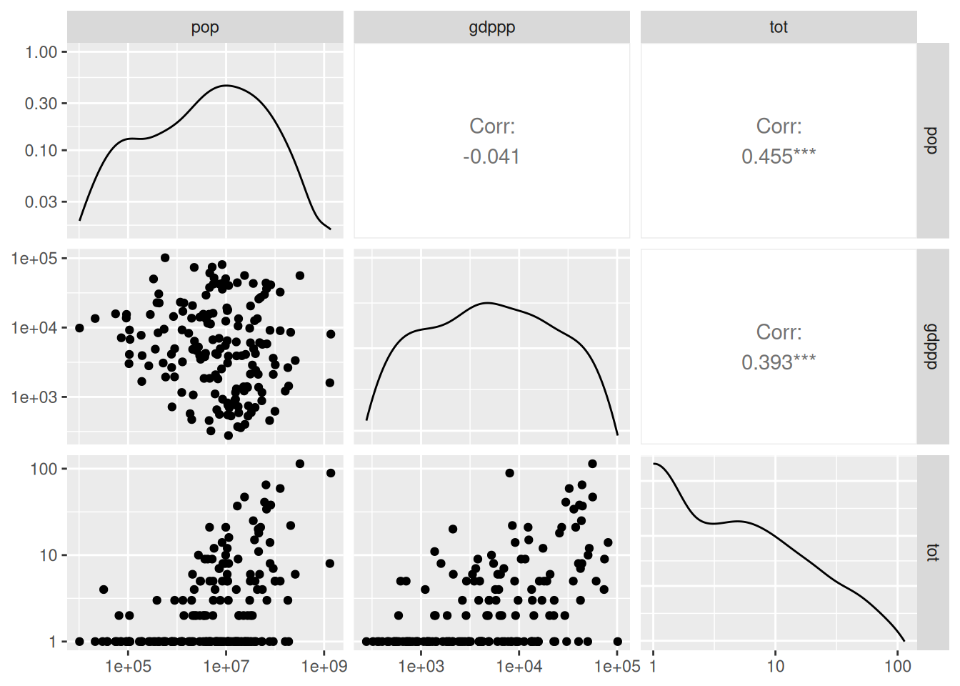
Data scientists working for the Guardian newspaper have compiled a data set, also made available via Kaggle, of population and GDP-per-capita (GDPpc) values for the majority of NOCs. From Figure 7, in which we plot this data, we observe significant positive correlations between population and medal count, and GDPpc and medal count.
Nielsen is a US media analytics company who publish predictions for the 30 NOCs with the highest medal counts. These predictions, which they refer to as the Gracenote Virtual Medal Table, are used to demonstrate the company’s capabilities both in terms of analysis and communication. Using the commentary accompanying the table as a guide, it appears that significant statistical effort and expert judgement has contributed to the predictions, making them a valuable resource. At least two of our forecasters made use of this data; either by computing a weighted average of their predicted medal counts and those of Nielsen, or by using discrepancies between their predictions and Gracenote’s to diagnose problems with their model.
A prediction that adopts the Gracenote ranking for the top 30 positions and ranks all other NOCs as tied at 31 leads to a tau score of approximately 0.252, below all of the competition’s entrants. Forecasting the 2024 ranking using the 2020 ranks gives us a tau of approximately 0.507. This is improved only slightly, to 0.511, by adopting the Nielsen Gracenote predictions for the top 30 NOCs while leaving the others in the 2020 ordering. These values serve as useful benchmarks when appraising our model-based forecasts in the next section.
| Code | NOC | Gold | Silver | Bronze | Total | Rank |
|---|---|---|---|---|---|---|
| USA | United States | 39 | 32 | 41 | 112 | 1 |
| CHN | China | 34 | 27 | 25 | 86 | 2 |
| FRA | France | 27 | 21 | 12 | 60 | 3 |
| GBR | Great Britain | 17 | 20 | 26 | 63 | 4 |
| NED | Netherlands | 16 | 10 | 8 | 34 | 5 |
| AUS | Australia | 15 | 23 | 16 | 54 | 6 |
| JPN | Japan | 13 | 13 | 21 | 47 | 7 |
| ITA | Italy | 11 | 19 | 16 | 46 | 8 |
| GER | Germany | 11 | 12 | 12 | 35 | 9 |
| KOR | South Korea | 9 | 4 | 13 | 26 | 10 |
| BRA | Brazil | 8 | 4 | 6 | 18 | 11 |
| CAN | Canada | 7 | 9 | 5 | 21 | 12 |
| HUN | Hungary | 7 | 6 | 7 | 20 | 13 |
| ETH | Ethiopia | 6 | 3 | 3 | 12 | 14 |
| ESP | Spain | 5 | 5 | 8 | 18 | 15 |
| DEN | Denmark | 5 | 5 | 4 | 14 | 16 |
| KEN | Kenya | 5 | 4 | 3 | 12 | 17 |
| TUR | Turkiye | 4 | 5 | 5 | 14 | 18 |
| NZL | New Zealand | 4 | 4 | 6 | 14 | 19 |
| SWE | Sweden | 4 | 4 | 4 | 12 | 20 |
| BEL | Belgium | 4 | 2 | 6 | 12 | 21 |
| IRI | Iran | 4 | 2 | 5 | 11 | 22 |
| POL | Poland | 3 | 7 | 7 | 17 | 23 |
| GEO | Georgia | 3 | 4 | 5 | 12 | 24 |
| UZB | Uzbekistan | 3 | 2 | 7 | 12 | 25 |
| UKR | Ukraine | 2 | 4 | 7 | 13 | 26 |
| IRL | Ireland | 2 | 3 | 5 | 10 | 27 |
| KAZ | Kazakhstan | 2 | 3 | 5 | 10 | 27 |
| JAM | Jamaica | 1 | 5 | 4 | 10 | 29 |
| SUI | Switzerland | 0 | 6 | 6 | 12 | 30 |
4 Poisson regression
4.1 Some comments
The Poisson regression model provides a convenient and well-studied device for predicting count data, and was adopted by several of our forecasters. It is worth noting, however, that the Poisson regression model does not naturally account for interaction effects between responses, such as the negative correlations that result from multiple NOCs competing for the same finite number of medals. This feature in our data could be accounted for using multinomial regression model. While R’s nnet package includes a function for fitting multinomial regression models, it is not easy to customize to our forecasting problem. More specifically, the package’s code would need to be modified if regression coefficients describing the dependence on future medal on covariates were to be shared by multiple NOCs.
One of our most successful forecasters did implement a different type of multinomial regression model - a binomial regression calculation in which the parameters of interest were the expected fraction of qualified athletes for each NOC who win a gold medal. This innovative modelling idea allowed the forecaster to leverage information about the 2024 games, namely the numbers of qualified athletes, that other forecasters would have found difficult to use. Having said this, the binomial model implicitly assumes that the (gold winning) success rate is independent of the number of (qualified athletes) trials. One can imagine problems with this assumption, however, if NOCs reduce the size of their contingent by selecting only their best athletes.
It is interesting to speculate whether accounting for both the number of qualified athletes for a particular NOC and the total number of medals available, both of which place upper bounds on the number of medals that can be won, would improve forecasts. The resulting regression model would presumably need to employ a variant of the mass function for the hypergeometric distribution as its likelihood function. Technically, this would take us outside the generalized linear model framework since the hypergeometric distribution falls outside the exponential family of distributions.
4.2 Covariate construction and selection
Since the target ranking is based predominantly on the number of gold medals won by each NOC, it seems sensible to use the gold medal count for an NOC at previous games to derive covariates for predicting the count at future games. We stand to benefit, however, from also accounting for good but not gold medal-winning performances. A convenient way to this is to add together contributions to a gold medal ‘pseudo-count’ that are calculated as a decreasing function of the rank achieved in an event. In the models fitted below we add up the reciprocals of ranks, excluding tied ranks which are seen often in knock-out events. This has the effect of producing a weighted medal count in which a second place (silver medal) is equivalent to half a gold, a third place (bronze medal) is equivalent to one third etc.
The candidate covariates for our Poisson model are:
2 lagged gold medal counts,
2 lagged sums of reciprocals of ranks achieved,
linear and quadratic terms in log population and log GDP per capita,
a dummy variable for the host nation.
To reduce the threat of overfitting we make use of R’s step function which, in our implementation, performs a backwards step-wise search over combinations of covariates, removing them one at a time until the AIC starts to rise. In this case the covariates related to population are removed, as is the lag-1 gold medal count. The degree to which meaning can or should be read into this covariate selection is another interesting issue. It suggests to us not that covariates like population are unrelated to gold medal counts but they they appear to contribute relatively little explanatory power once the other covariates have been accounted for. We are aware of the existence in the literature of criticisms, such as Thompson (1995), of stepwise regression procedures in the context of explanatory analyses - warning us not to read too much into the presence or absence of covariates in the final model. We are also aware of authors, such as Subramanian and Simon (2013), who claim that penalized regression methods are preferable to stepwise regression methods for predictive modelling on the basis that the latter generally do not reduce sampling variance enough. While not refuting their claims, we note here that the stepwise model selection does modestly improve our forecasts for the (out of sample) 2024 counts from a tau of 0.558 to 0.562.
Adjusting the expected medal counts given the absence of Russia, assuming that they would win 20 gold medals as they did in 2020 which are redistributed over the remaining countries, takes our tau score up to 0.571. If we now bring in the Gracenote predictions, using them to identify and order the top 30 NOCs, below which we use ranking based on our own expected medal count, we increase our tau score again to 0.574. We are now approaching the top of the forecaster leader board and doing so without the benefit of bookmakers’ odds. We are still, however, a fair distance from the champion forecaster.
4.3 XGBoost
The simple Poisson regression model appears to fit the data well but it is interesting to ask whether this 20th-century model can be improved upon using more contemporary machine learning techniques. Specifically, we now (briefly) investigate the applicability of gradient boosted tree models that assign different Poisson rate parameters to regions of the covariate space. These models have proved to be highly popular among statisticians, data scientists and machine learners, partly due to their predictive performance on large, complex data sets and partly due to the ease with which they can be fitted using open source software such as the python package XGBoost. A thorough description of gradient boosted trees is beyond the scope of this report. The paper from Chen and Guestrin (2016), which accompanies the XGBoost package provides information on the ideas and computations involved.
The gbm package (Ridgeway and Developers (2024)) for R provides many of the model fitting functions that have made XGBoost so popular, including those for Poisson regression and ranking problems. The gradient boosted Poisson model quickly and easily produced for us a set of expected gold medal counts whose implied ranking leads to a tau score of 0.556, which we view as being almost negligibly different from the score of the simple Poisson regression model of the previous section. The gradient boosted tree that specifically optimizes the Kendall’s tau for previous games leads to a prediction that scores a tau score of 0.557 for the 2024 games. While acknowledging the dangers of over-interpreting these numbers, they suggest to us that neither the move to gradient boosted tree models nor the adoption of the rank-based loss function for model fitting greatly improve performance beyond that of the simpler Poisson regression model.
5 Disaggregated poisson regression
5.1 Disaggregation by NOC
One of our highest scoring forecasters began their modelling efforts by first clustering the NOCs (into 5 groups) based on their historical medal counts. Ordinary least squares, rather than Poisson regression, was used to fit and predict for each group and ranks computed from those predictions. This approach fits well with the idea that different NOCs employ different strategies when assembling and training their Olympic teams. It could also be seen as a response to the earlier observation that different NOCs appear to target different sets of disciplines, whose medal counts are characterized by distinct behaviours.
5.2 Disaggregation by discipline
We now investigate whether separately modeling medal counts for subsets of the Olympic disciplines provides a way for us to improve our predictions. Fitting multiple models clearly increases the total number of parameters to be estimated and so leaves us more vulnerable to overfitting. The problem is particularly severe when we consider disciplines dominated by a small number of NOCs, whose previously observed medal counts effectively determine estimated regression coefficients while the non-dominating NOCs have little to no influence. At the risk of labouring the point, the NOCs winning no gold medals are informative for regions of the covariate space associated with low expected medal counts but not for the relative lowness of expectations within that region.
One modelling strategy that may help to alleviate this problem is to disaggregate by discipline only partially. It is conceivable that a carefully constructed hierarchical model could be constructed so that parameters relating to different disciplines are shared to a greater or lesser degree depending on their proximity in a (pre-specified) tree structure. Theory (Gelman (2007)) and software (Bates et al. (2015)) exist to guide such a modeling exercise but it is likely to require considerable care. A simpler approach would be to cluster disciplines and fit independent models to medal counts for each one. We did not attempt this but believe that it could work well.
6 Appraising the submissions
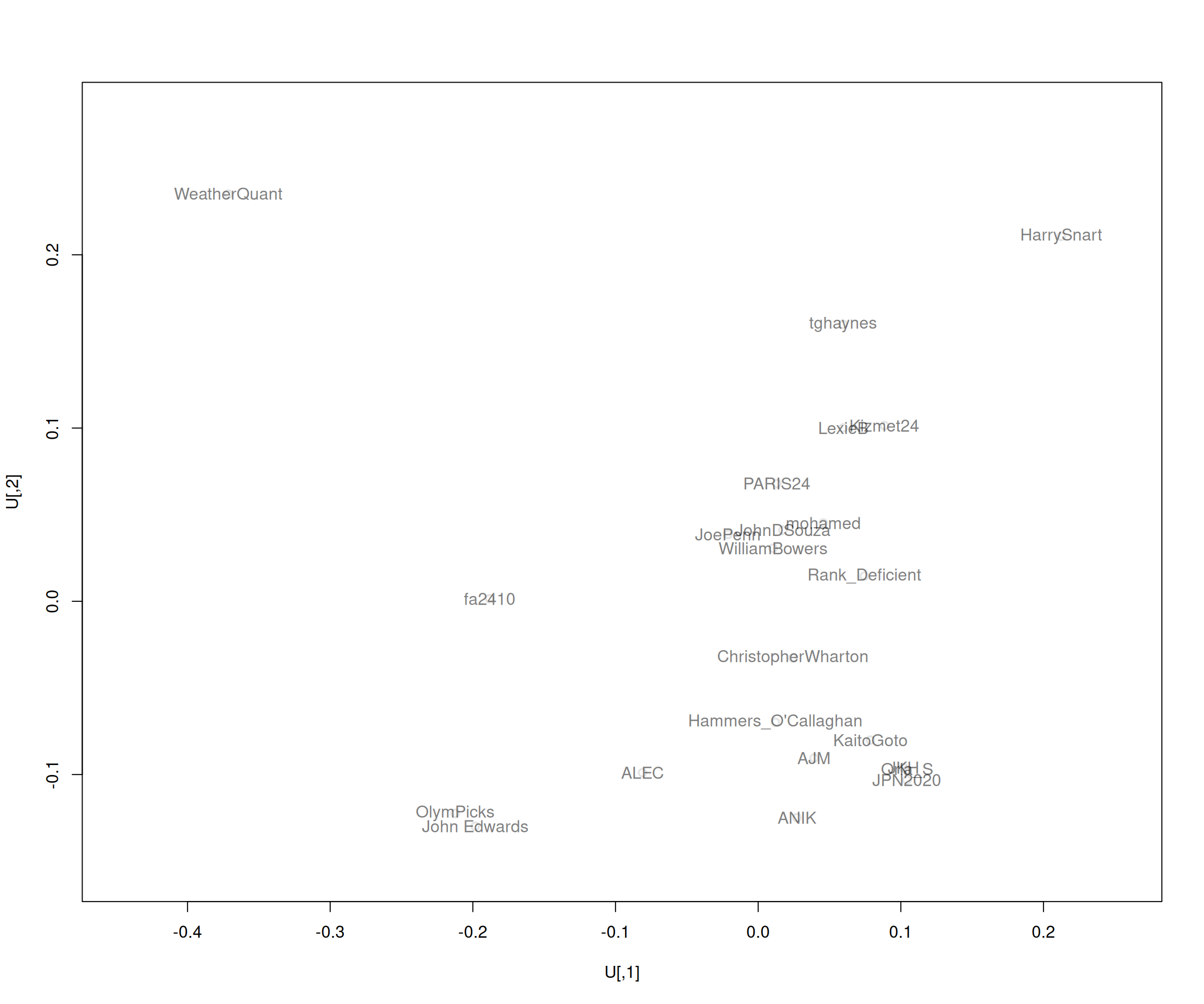
We can visualize the forecasters’ predictions by embedding them in two dimensions. The process chosen for doing so in Figure 8, below, is a standard metric multidimensional scaling calculation, which involves the eigen-decomposition of a centred squared distance matrix. In this case our distances are defined by subtracting from one the Kendall’s tau correlation between pairs of forecasts. We notice from the plotted embeddings that forecasters Orla and JKH appear to have stuck quite closely to the ranking from the Japan 2020 Olympics and that two of our best forecasters, John Edwards and Olympicks, may have ended up with relatively similar forecasts via different means.
The true observed NOC ranking in also included in Figure 8 and, interestingly, its distance in the embedding to the forecasted rankings is not really representative of the scores of the forecasts. It appears that the forecast-to-forecast distances are effectively prioritized over the forecast-to-truth distances in the MDS calculation and there is not a two-dimensional embedding that capture both well. With this observation we note that visualization of ranking data remains a challenge and that, perhaps, 2-dimensional embeddings are ill-suited to the task. In Figure 9 we try a different approach, plotting a heatmap illustrating the tau correlations between the forecasters. The brightest yellow cells on the diagonal correspond to forecasters who assigned different ranks to all NOCs, while the dark blues correspond to those who forecast a large number of ties. A relatively bright cell at the intersection of the row and column for John Edwards and Olympicks again shows the similarity of their forecasts. We also see relatively dark rows for Lexie B and Mohamed, suggesting that their forecasts and, presumably forecasting methods, were dissimilar to the others.
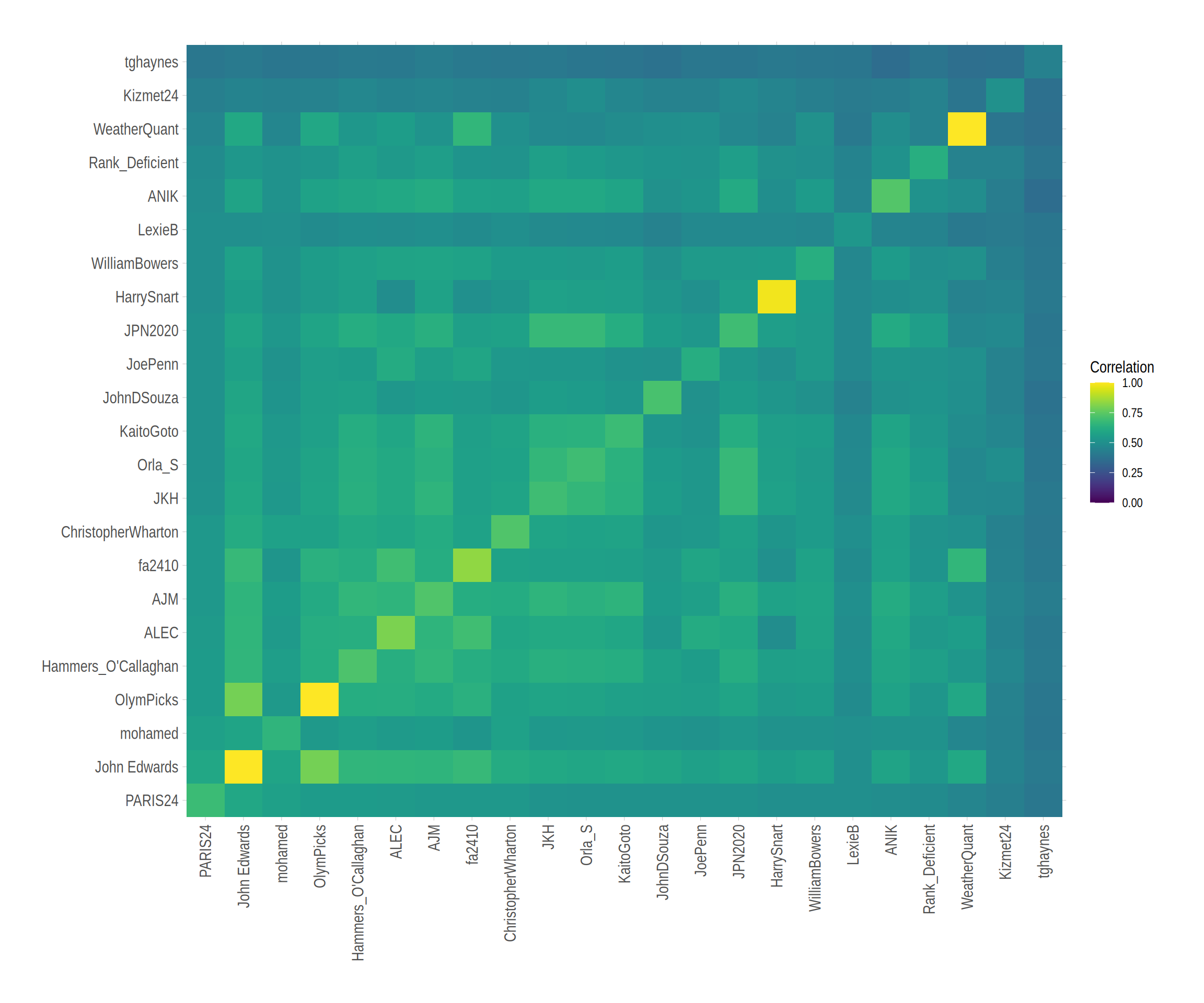
The final ranking based on the Kendall’s tau correlations between forecasts and the actual 2024 gold medals table is presented below. As noted above, our own Poisson regression model (with Gracenote and Russian-absence corrections) scored 0.574 which would have put us in second place, behind our champion John Edwards whose forecasting strategy is briefly described in Section 7.
| Forecaster | Rank | Tau |
|---|---|---|
| John Edwards | 1 | 0.596 |
| mohamed | 2 | 0.564 |
| OlymPicks | 3 | 0.544 |
| Hammers_O’Callaghan | 4 | 0.543 |
| ALEC | 5 | 0.540 |
| AJM | 6 | 0.534 |
| fa2410 | 7 | 0.533 |
| ChristopherWharton | 8 | 0.532 |
| JKH | 9 | 0.513 |
| Orla_S | 10 | 0.511 |
| KaitoGoto | 11 | 0.509 |
| JoePenn | 13 | 0.508 |
| JohnDSouza | 13 | 0.508 |
| JPN2020 | 14 | 0.507 |
| HarrySnart | 16 | 0.495 |
| WilliamBowers | 16 | 0.495 |
| LexieB | 17 | 0.493 |
| ANIK | 18 | 0.486 |
| Rank_Deficient | 19 | 0.480 |
| WeatherQuant | 20 | 0.455 |
| Kizmet24 | 21 | 0.426 |
| tghaynes | 22 | 0.395 |
Following discussions with some of the competition entrants it became clear that several low-scoring forecasts were the result of over-fitted models and to aggressive optimization of the wrong metric. Specifically, one entrant had fitted a model to optimize a variant of the standard Kendall’s tau known as \(\tau_b\) and defined as\[ \tau_b(\hat R, R) = \frac{\tau(\hat R, R)}{\sqrt{\tau(\hat R, \hat R)\tau(R,R)}} \] The distinguishing feature of this statistic is the \(\sqrt{\tau(\hat R,\hat R)}\) in the denominator that effectively rewards the specification of ties. In the extreme case, in which a forecast predicts ties for all items, \(\tau(\hat R,\hat R)=0\) and \(\tau (\hat R,R)\) become infinitely large. While this extreme behaviour is clearly undesirable, it is interesting to consider whether and how modifications to the scoring metric would have changed the results of our competition. Although we do not present the results here, we can confirm that changing the metric to \(\tau_b\) changes the results significantly, with several of the best scoring forecasters being sent almost to the bottom of the leader board and at least one forecaster towards the bottom rising to the top third.
It could be argued that a metric like \(\tau_b\) is more suitable for future forecasting competitions than \(\tau\), which tends to reward forecasters who assign unique ranks to all items. This is because assigning unique ranks to a large number of items may only be possible for entrants with relatively advanced computational skills and resources. To a degree, this shuts out school-age entrants and entrants with valuable domain knowledge but limited technical training. It would be nice for the competition to recognize these types of entrants, and the organizers will certainly keep this in mind when designing next year’s competition.
7 John Edwards
John Edwards won our forecasting competition. His modelling strategy involved using gradient boosted trees to predict the likely winner of each Olympic event given the numbers of medals won and athletes entered by the NOCs. The predictions arising from this model were overwritten by implied probabilities from bookmaker’s odds when they were available. John proceeded to use the NOCs’ relative gold-winning probabilities to infer their relative strengths from which he could compute probabilities for silver and bronze medals. A final step in producing his ranking involved rounding expected aggregated gold, silver and bronze medal counts and sorting them in the same (lexographic) way as the Olympic medals table. Approximately 64% of pairs of NOCs are correctly ordered in John’s predicted ranking, only 4% are in the incorrect order and 32% are tied so are considered neither right nor wrong.
John’s high tau score appears to be the result of multiple factors, many of which are inter-related. Perhaps the most important was the choice to model medal counts at the level of events. This allowed for the direct use extra information from bookmakers, which characterized the entries from both of our competition’s top-scoring forecasters. The gradient boosted trees, with their distinctive variable selection process at each iteration, appear to have useful for avoiding overfitting. This is particularly important when only a relatively small amount of the most recent data is used to fit models.
A more comprehensive description of John’s entry is provided on his website.
8 Conclusions and remarks
We end with a few concluding remarks, which really act as a list of things to remember for the competition organizers but may also be of interest to the readers of this blog.
8.1 Insights into statistical methodology
- The Poisson model for gold medals using previous medal counts and demographic data as covariates produced a good ‘base prediction’ for us to build on.
- The greatest improvements on this base prediction came from adjustments made in response to information extraneous to the Poisson model’s training data, specifically the adjustments relating to Russia’s absence and to the insights from the Gracenote forecasters. Increasing model sophistication while using the same data, by using a gradient boosted tree model rather than a simpler generalized linear model, tended to lead to incremental improvements to forecast accuracy. Having said that, incremental improvements can still be valuable in the context of a forecasting competition like ours.
- The implications of the treatment of ties by Kendall’s tau ought to have been more clearly described to forecasters. The vanilla version of Kendall’s tau, which we employed, effectively rewarded forecasters for exaggerating the differences between NOCs. More precisely, it incentivized forecasters to predict distinct ranks for a pair of NOCs even if the (forecaster’s) probability of a tie was very high.
- More data for model fitting is unarguably a good thing when we can be confident that that data is relevant to what we want to estimate or forecast. When we look back in time for data to inform time series-type models, however, we open ourselves up data artefacts that can fatally undermine inferences. In our case zero counts due to boycotts in the 1980 could have severely negatively affected forecasts.
- It remains unclear to us, in the context of modelling count data, how much predictive power could be improved by disaggregating those counts. Total enumeration of partial disaggregations is clearly computationally intractable but it may be interesting to look at a few via greedy stepwise search, analogous to those used in hierarchical clustering.
8.2 Insights into the Olympics
- China has a very high proportion of golds given the number of athletes competing.
- It appears that the home advantage is just down to bringing more athletes. The fraction of golds does not seem to be effected.
- Russia’s absence in the 2024 Olympics affected the medals table. More specifically, it appears to have boosted the medal counts for NOCs further down the medals table who, historically, tended to win medals in the disciplines Russia also won medals in.