Call:
glm(formula = glmy ~ glmx, family = "binomial")

Coefficients:
            Estimate Std. Error z value Pr(>|z|)
(Intercept) -0.30416    0.04229  -7.192 6.38e-13 ***
glmx         0.53767    0.04126  13.031  < 2e-16 ***
---
Signif. codes:  0 '***' 0.001 '**' 0.01 '*' 0.05 '.' 0.1 ' ' 1

(Dispersion parameter for binomial family taken to be 1)

    Null deviance: 3384.5  on 2476  degrees of freedom
Residual deviance: 3195.5  on 2475  degrees of freedom
AIC: 3199.5

Number of Fisher Scoring iterations: 4QSA:Y blog
On this page you will find some jottings from our group’s members on topics they find interesting.
Elo and its variants
Ben Powell - 3 Nov 2023.
What is the Elo system for rating teams, and why does it matter? The Elo system is cool because it means different things to different people. It is simultaneously a set of rules for assigning scores to teams and a probabilistic model for interpreting and predicting outcomes. Predictive power is obviously a key feature but so is the intelligibility of the model, whose parameters effectively provide us with a language with which we can talk about teams and their performance.
Basic Elo
The Elo system for scoring players and predicting the outcomes of competitions is an important and well known tool for sports analysts. Originally developed for the chess community, the system has been modified and extended significantly for different applications. The most basic version involves allocating a parameter to each player that serves to quantify their strength or ability. When two players compete with each other the difference between their parameters is used to determine the probability that one will beat the other. For example, consider players labelled \(i\) and \(j\) with strength parameters \(R_i\) and \(R_j\). According to the Elo system, the probability that player \(i\) beats \(j\) in a match is
\[ P(\text{i beats j})=\frac{1}{1+e^{-(R_i-R_j)}}. \]
Going from strength parameters to probabilities is easy. The tricky bit is to estimate strength parameters given observed outcomes of matches. Typically the parameters are adjusted incrementally as each match outcome is instantiated. The adjustment is made to move the parameters in the direction of the gradient of their log-likelihood (the log-probability of having observed the outcome). This leads us to the following adjustment equations
\[\begin{align*} R_i \gets R_i + \gamma \left[ \ \mathbb{1}(\text{i beats j})-P(\text{i beats j}) \ \right],\\ R_j \gets R_j - \gamma \left[ \ \mathbb{1}(\text{i beats j})-P(\text{i beats j}) \ \right] \end{align*}\]
where the left-pointing arrow signifies updating the left-hand quantities with the right-hand ones, the quantity \(\mathbb{1}( \cdot)\) is a binary indicator function taking value one when its argument is true and zero otherwise and \(\gamma\) is a scalar step-size hyperparameter.
Having established the basics, there are lots of ways to modify the Elo system. We can, for example, play around with the step-size parameter so that we make big adjustments for new players (and so infer more about their relative strength from each game) and less for experienced players (whose strength we may already be fairly sure about). We can extend the system to account for draws, for the fact that their may be more that two players in a competition or to account for the fact that a one-dimensional representation of strength may be too simplistic.
Elo + goal difference
For chess the outcome is everything. It doesn’t matter if you lost lots of powerful pieces in order to win. The win is all that matters… this might be a slight over simplification because we can sometimes appreciate that a game was won with flair or grace, but these qualities arguably defy easy quantification.
For football it is easier to see that the circumstances of a (win/draw/lose) outcome do provide additional usable information regarding the teams’ relative abilities. The goal difference at full time is an obvious example of such information. In this section we discuss one way to extend the Elo scoring system to account for it.
Model specification
Our approach involves the adoption of a two-stage model for a match’s outcome. The first stage is usefully referred to as an Elo-Davidson model. This is Davidson’s extension of Elo’s model, which accommodates draws (see Davidson (1970)). In the second stage we model the goal difference given the match result using a Poisson distribution. More precisely, we consider a match for which the difference between strength parameters for the home and away teams is \(D=R_H-R_A\), and the number of goals scored by the home and away teams are \(G_H\) and \(G_A\), respectively. The probabilities for the match outcomes are
\[\begin{align*} P(\text{Home win})= \frac{e^{D}}{e^{D}+e^{u+vD}+1},\\ P(\text{Draw})= \frac{e^{u+vD}}{e^{D}+e^{u+vD}+1},\\ P(\text{Away win})= \frac{1}{e^{D}+e^{u+vD}+1}, \end{align*}\]
Then, conditional on the match outcome we model the goal difference as
\[\begin{align*} |G_H-G_A|-1 \sim \begin{cases} \text{Poisson}(\lambda=e^{a+bD}) & \text{Home win}\\ \text{Poisson}(\lambda=e^{a-bD}) & \text{Away win}\\ -1 & \text{Draw} \end{cases} \end{align*}\]
This Poisson model is a way to formalize the idea that if a good home team beats a bad away team, then we expect the goal difference to be large. And if a good home team loses to a bad away team, we expect the goal difference to be small. The words ‘good home team’ and ‘bad away team’ here correspond to the case in which \(R_H \gg R_A\) so that \(D \gg 0\).
The component distributions in the model above are all highly standard. It is only really the specific composition that is novel here. Our model is designed so that the match (win/draw/lose) results and their probabilities are of paramount importance. The numbers of goals scored are considered afterwards and, in a sense, add supplementary information about a match. This modelling approach differs from the one put forward by Dixon and Coles (Dixon and Coles (1997)), who begin by directly (i.e. not conditional on the match result) modelling the distributions for the numbers of goals scored and derive result probabilities from these distributions.
(Hyper-)parameter specification
We now need to specify suitable values for the model parameters, starting with the Elo-Davidson component. We are going to be a bit sneaky here and make use of some bookmaker’s odds. For a given match the log odds for a home win over an away win tell us the bookmaker’s estimate for \(D\) and the log odds for a draw over an away win tell us about their estimate for \(u+vD\). One way to proceed would be to fit a linear model to the two sets of bookmaker’s log odds, and so infer their beliefs about \(u\) and \(v\). Alternatively, we can compute the bookmakers \(D\) values and fit a logistic regression model to the draws (when we consider the population of matches for which a home win does not occur).
We fit this logistic regression model and ask R to produce a summary.
The MLE computed here suggests to us that \(u \approx -0.3\) and \(v \approx 0.5\) are suitable parameter values for our model.
Now let’s consider the Poisson model parameters \(a\) and \(b\). We use R to fit a Poisson regression model for which the response variables are the goal differences (minus one) for the matches that do not result in a draw, and the covariates are bookie-estimated \(D\) strength differences (with the sign flipped when the away team wins). The fitted model summary looks like this.
Call:
glm(formula = glmy ~ glmx, family = "poisson")

Coefficients:
            Estimate Std. Error z value Pr(>|z|)
(Intercept) -0.39912    0.02525  -15.81   <2e-16 ***
glmx         0.30279    0.01645   18.41   <2e-16 ***
---
Signif. codes:  0 '***' 0.001 '**' 0.01 '*' 0.05 '.' 0.1 ' ' 1

(Dispersion parameter for poisson family taken to be 1)

    Null deviance: 4844.3  on 3438  degrees of freedom
Residual deviance: 4496.2  on 3437  degrees of freedom
AIC: 8671.3

Number of Fisher Scoring iterations: 5
The GLM fitting routine in R identifies a significant relationship between the goal differences and the team strength differences, which is reassuring. The MLE it computes indicates that \(a \approx -0.4\) and \(b \approx 0.3\) are suitable values for the model parameters.
Inference and prediction
We now think about how the model can inform our inferences for the team strengths \(R_i\), where the subscript \(i\) labels the teams. We choose to use the strategy adopted in the Elo system and make adjustments to the \(R_i\) by moving them incrementally in the direction of the gradient of the log-likelihood induced by our model. This results in the follow algorithm for parameter updates:
Suppose the home team receives \(1\) point for a win, \(v=0.5\) points for a draw and \(0\) points for a loss. The Elo-Davidson part of the model tells us to adjust the home teams strength parameter in the direction of the difference between the actual and expected points received, i.e.
\[\begin{align*} R_H \gets R_H + \gamma \ \left[ Q-E(Q) \right],\\ R_A \gets R_A - \gamma \ \left[ Q-E(Q) \right]. \end{align*}\]
where \(Q\) denotes the points received by the home team
\[\begin{align*} Q= \begin{cases} 1 & \text{Home win},\\ v & \text{Draw},\\ 0 & \text{Away win} \end{cases} \end{align*}\]
and
\[\begin{align*} E(Q)=\frac{e^D+ve^{u+vD}}{e^D+e^{u+vD}+1} \end{align*}\]
and \(D=R_H-R_A\).
The next part of the algorithm involves an update given the observed goal difference. Again, it takes the form of an adjustment in the direction of the difference between observed and expected quantities.
\[\begin{align*} R_H \gets R_H + \gamma \ b \ \text{sign}(S) \ \left[ |S|-E(|S|) \right],\\ R_A \gets R_A - \gamma \ b \ \text{sign}(S) \ \left[ |S|-E(|S|) \right]. \end{align*}\]
where
\[\begin{align*} S=G_H-G_A,&& E(|S|)=\exp \left( a+b \ \text{sign}(S) \ D \right)+1 \end{align*}\]
and we have used the convention
\[\begin{align*} \text{sign}(S) = \begin{cases} 1 & S>0\\ 0 & S=0\\ -1 & S<0 \end{cases} \end{align*}\]
Tests
Let’s take a look at how our extended Elo-type algorithm works on some real data, specifically on match results from the English Premier League at around the time of writing.
The data is stored in a data frame named EPL23
Code
head(EPL23) Date HomeTeam AwayTeam FTHG FTAG FTR
1 2023-08-11 Burnley Man City 0 3 A
2 2023-08-12 Arsenal Nott'm Forest 2 1 H
3 2023-08-12 Bournemouth West Ham 1 1 D
4 2023-08-12 Brighton Luton 4 1 H
5 2023-08-12 Everton Fulham 0 1 A
6 2023-08-12 Sheffield United Crystal Palace 0 1 AThe code chunk below implements our Elo-type algorithm and produces a plot of the estimated \(R\) parameters over time.
Code
N<-nrow(EPL23)
teams<-sort(unique(EPL23$HomeTeam))
M<-length(teams)
Rmatrix<-matrix(0,N,M)
colnames(Rmatrix)<-teams
u<--0.3;v<-0.5;a<--0.4;b<-0.3
gamma<-0.1

for(i in 1:(N-1)){
 homeind<-which(EPL23$HomeTeam[i]==teams)
 awayind<-which(EPL23$AwayTeam[i]==teams)

 D<-Rmatrix[i,homeind]-Rmatrix[i,awayind]
 Q<-as.numeric(EPL23$FTR[i]=="H")+v*as.numeric(EPL23$FTR[i]=="D")
 EQ<-(exp(D)+v*exp(u+v*D))/(exp(D)+exp(u+v*D)+1)
 delta<-gamma*(Q-EQ)

 S<-EPL23$FTHG[i]-EPL23$FTAG[i]
 EabsS<-exp(a+sign(S)*b*D)+1
 delta<-delta+gamma*b*sign(S)*(abs(S)-EabsS)

 Rmatrix[i+1,]<-Rmatrix[i,]
 Rmatrix[i+1,homeind]<-Rmatrix[i+1,homeind]+delta
 Rmatrix[i+1,awayind]<-Rmatrix[i+1,awayind]-delta
}

laby<-seq(min(Rmatrix[N,]),max(Rmatrix[N,]),length=M)[rank(Rmatrix[N,])]

plot(EPL23$Date,rep(0,N),ylim=range(Rmatrix),xlim=c(min(EPL23$Date),max(EPL23$Date)+24),col=0,ylab="R params",xlab="Date");for(i in 1:M){points(EPL23$Date,Rmatrix[,i],type="o",lwd=2,col=mypal[i%%length(mypal)+1])};text(rep(EPL23$Date[N]+2,M),laby,labels=teams,pos=4);for(i in 1:M){points(EPL23$Date[N]+c(0,2),c(Rmatrix[N,i],laby[i]),type="l",lty=2,col=rgb(0,0,0,0.5))}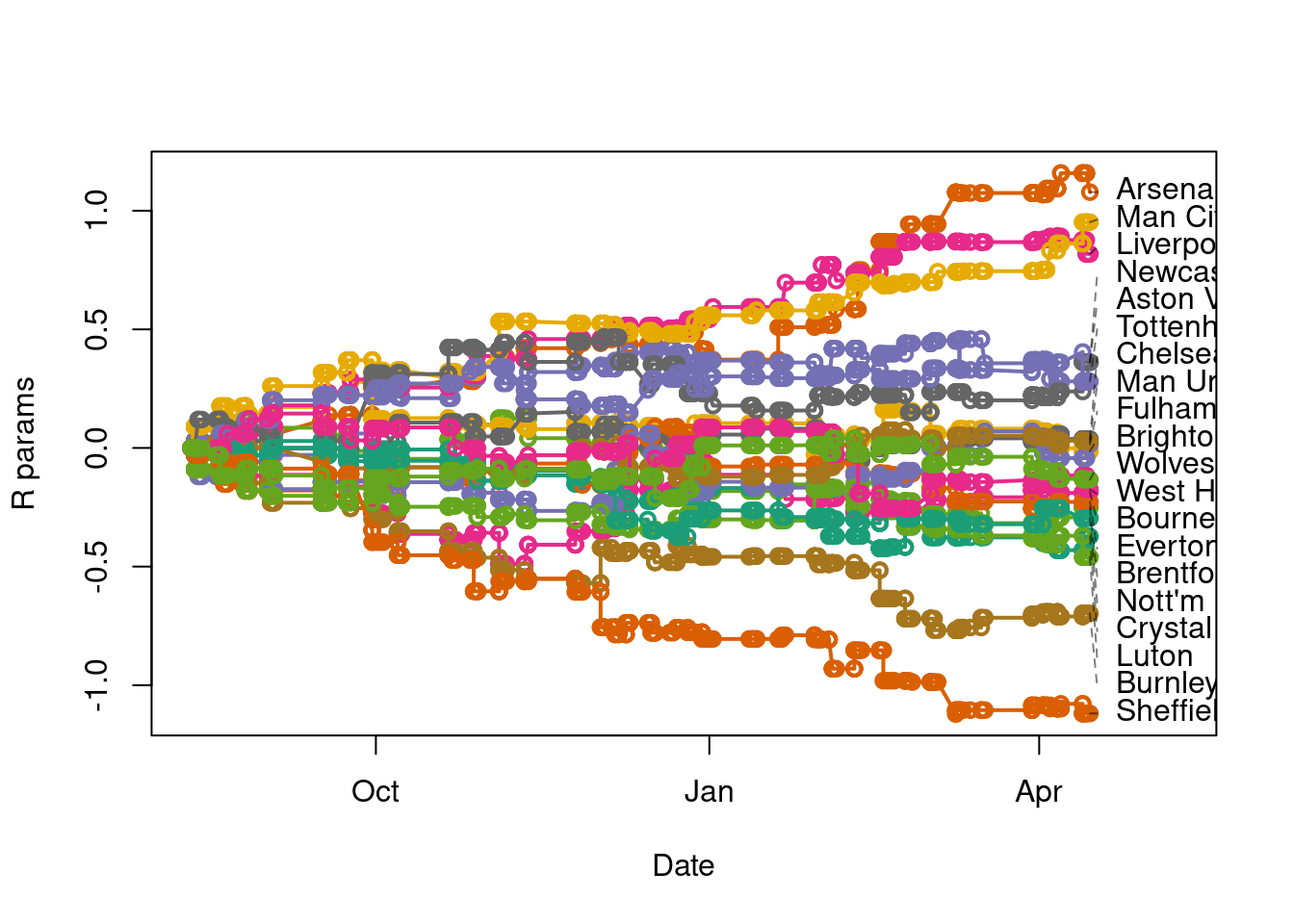
This preliminary calculation shows us that the model is working reasonably well insofar as leading to a ranking of teams in approximate agreement with the league table. This post has already become rather long so I will reserve further analysis and exposition for another time. An important next step, for example, is to think about ways to initialize the \(R\) parameters at the beginning of the season which might involve analysis of previous seasons or of probabilities implied by betting markets.
Discussion
Experimenting with the ‘Elo + goal difference’ model is fun, but is it worthwhile? Arguably, it could be considered as a case of ‘messing with a classic’ like adding extra spoilers to a classic car or sprinkling hundreds-and-thousands on an apple crumble. Sometimes less is more, especially when the simplicity of an idea is key to it attaining significance and meaning within a community. The message I think we can take away is that Elo-type models can be adapted to accommodate more than just match outcome data. The extent to which supplementary data can inform predictions of future outcomes ought to be considered theoretically and tested empirically (which I have not done in this blog post). Theoretical arguments could be formulated via the analysis of the Fisher Information for strength parameters that is contributed by supplementary data and empirical tests will be most convincing if the accuracy of our predictions exceeds certain benchmarks, specifically the benchmarks set by bookmakers.
References
Davidson, Roger R. 1970. “On Extending the Bradley-Terry Model to Accommodate Ties in Paired Comparison Experiments.” Journal of the American Statistical Association 65 (329): 317–28.
Dixon, Mark J, and Stuart G Coles. 1997. “Modelling Association Football Scores and Inefficiencies in the Football Betting Market.” Journal of the Royal Statistical Society: Series C (Applied Statistics) 46 (2): 265–80.