1.6. The Heisenberg uncertainty principle

1.6.1. Position momentum form of the uncertainty principle

The Heisenberg uncertainty principle tells us that the precision with which we can know the position and momentum of a particle has a fundamental limit. In its mathematical form is states

(1.12)\[ \delta x \delta p \ge \frac{\hbar}{2} \]

where \(\delta x\) and \(\delta p\) are the uncertainties in the position and momentum, respectively. This has implications for how well we can measure both of these numbers simultaneously. Consider figure 1.16 due to my very poor photography skills I have many blurred pictures of my dog (Tam-Tam the quantum hound). From the picture we can give Tam’s position with some uncertainty, assuming she moves with a constant velocity it will be related to the width of the position distribution given at the top of the picture. If we know the shutter speed of the camera we can say something about Tam’s velocity and hence her momentum. By adjusting the shutter speed of my camera I can trade knowledge of her position for knowledge of her momentum, one gets worse as the other improves. In the quantum world the uncertainty in position and momentum are related by equation (1.12).

A fundamental limit

You should note carefully unlike with the example using my poor photography this is not a consequence of errors in the experimental measurement this is a fundamental limit placed on this measurement by the wave nature of particles.

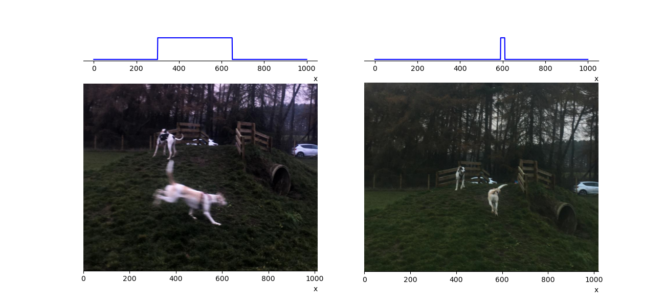
Fig. 1.16 In the left picture Tam has an uncertain position due to my poor photograph skills, we can estimate her momentum by knowing the camera’s shutter speed but only at the expense of precision in her position. In the right picture Tam is moving slower, we learn about her position but any estimate of momentum would be worse. The upper panels are a schematic representation of Tam’s position. Their width is related to any uncertainty in her position.

How do we know Tam isn’t a quantum object?

When passed through a single slit she does not diffract.

1.6.2. Energy time form of the uncertainty principle

The Heisenberg uncertainty principle has many forms, later in your degree you will learn how these are related to pairs of observable quantities. However, you need to learn quite a bit more quantum physics before that happens. For now will will introduce just one other form, the energy-time Heisenberg uncertainty principle. It is simple to derive this from the momentum-position form, recall that we are working with uncertainties. First we need to relate small changes in \(E\) to small changes in \(p\)

\[\begin{split} \frac{\delta E}{\delta p}&\approx\frac{dE}{dp}=\dfrac{d}{dp}\left( \frac{p^2}{2m} \right )\\ &=\frac{p}{m}=v=\frac{dx}{dt},\\ \delta p &\approx \delta E \frac{\delta t}{\delta x}. \end{split}\]

Substitute this equation into equation (1.12) to obtain

\[ \delta E \frac{\delta t}{\delta x} \delta x \ge \frac{\hbar}{2}. \]

Simplifying the expression leads to the energy-time form of the Heisenberg uncertainty principle

(1.13)\[ \delta E \delta t \ge \frac{\hbar}{2}. \]

Where \(\delta E\) and \(\delta t\) are the uncertainty in Energy and time, respectively.

1.6.3. Electron diffraction, de Broglie waves, and the Uncertainty principle

The amplitude of a wave propagating along the x-axis may be described by the equation

(1.14)\[ A=A_0 e^{i(k_x x-\omega t)} \]

where \(k_x\) is the wave number, \(x\) is the position, \(\omega\) is the angular frequency, and \(t\) is the time.

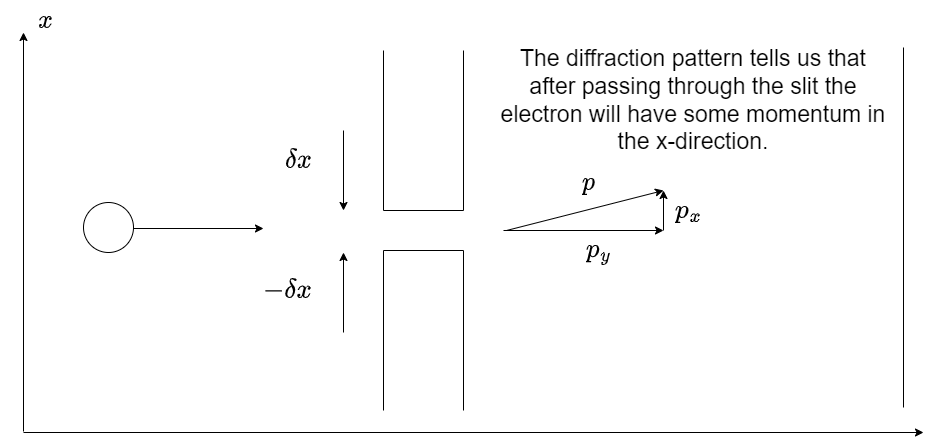
Fig. 1.17 A schematic of electron single slit diffraction. The electron must gain a momentum in the x-direction after the slit to allow the formation of a diffraction pattern.

Consider a coherent beam of electrons propagating towards a slit as shown in figure 1.17. The de Broglie equation (1.11) tells us that the electrons have a wavelength that is inversely proportional to their momentum, and the Einstein relationship \(E=h f\) relates the energy of our electrons to a frequency. We may relate \(k\) and \(\omega\) in equation (1.14) to the momentum \(p\) and energy \(E\) of the electrons,

(1.15)\[\begin{split} A&=A_0e^{i(k_x x-\omega t)}\\ &=A_0e^{i\left(\frac{2\pi}{\lambda_x}x-2\pi f t\right)}\\ &=A_0e^{i\left(\frac{p_x}{\hbar}x-\frac{E}{\hbar}t\right)}. \end{split}\]

If the beam of electrons is propagating in the \(y\) direction then before entering the slit the momentum in the \(x\) direction is zero. When passing through the slit we will in effect be making a measurement of the position to somewhere within the slit. According the the Heisenberg uncertainty principle given by equation (1.12) there will also be a related uncertainty in the momentum.

Let us say the slit is centred at \(x=0\) and extends \(\pm \delta x\) in either direction. Passing the electrons through the slit is an attempt to measure their \(x\) position. As the electron passes through the slit their de Broglie wave, given by equation (1.15), can now only have values of \(x\) from \(-\delta x\) to \(+\delta x\). We also know that in order for an electron to be diffracted by the slit the electron must have a momentum in the \(x\)-direction after it has passed through the slit (\(p_x\)). The size of the \(x\)-momentum will increase in magnitude as the angle \(\theta\) increases.

The de Broglie waves that travel from the top of the slit to the screen will traverse a different length path than those that travel to the screen from the bottom of the slit. Hence, there will be a path difference determined by the \(x\)-position on the screen. As the distance to the screen is fixed \(y\) and if we assume the screen distance is sufficently large that the small angle approximation is valid for sine then it will not contribute to the path difference in this example. Our electron is modelled by a de Broglie wave which is to a good approximation a superposition of de Broglie waves emitted across the width of the slit. We can create this superposition by integrating, we will also assume time \(t=0\),

(1.16)\[\begin{split} A&=A_0\int_{-\delta x}^{+\delta x} e^{i\left(\frac{p_x}{\hbar}x\right)} dx \\ &=A_0 \left[ \frac{\hbar e^{i \left(\frac{p_x}{\hbar}x\right)}}{i p_x} \right]_{-\delta x}^{+\delta x}\\ &=2 A_0 \hbar \frac{\sin(\frac{\delta x}{\hbar} p_x)}{p_x}. \end{split}\]

A plot of equation (1.16) squared is given in figure 1.18. The plotted function looks very much like the one you would expect for a single slit diffraction with a wave source. This is of course to be expected, in treating our electrons like waves and measuring their position we introduced an uncertainty into their momentum. This is manifested as a diffraction pattern, i.e. once the electrons pass through the slit their momentum in the x direction becomes uncertain. If we try be reducing the slit width then the width of the central maximum in the diffraction pattern would get wider making the momentum more uncertain. This is the behaviour predicted by the Heisenberg uncertainty principle.

Diffraction patterns

In figure 1.18 is plotted the superposition for a set of de Broglie waves. Note, as with diffraction patterns for wave sources what we would observe is the square of the function given in equation in (1.16). For now this doesn’t matter too much but we will pick this idea up later when we introduce the wave function and it’s probability density function. The key point is that de Broglie wave diffract in an analogous was to EM waves.

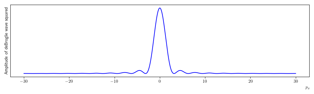
Fig. 1.18 A plot of equation (1.16) squared. The amplitude of the de Brolgie wave is plotted on the y-axis and is a superposition of de Broglie waves covering the whole slit width, the x-axis is the momentum in the x-direction. Notice that this looks very similar to the expected pattern for single slit diffraction with light. We can interpret the plot as the probability an electron will have a particular value of x momentum after passing through the slit. Hence, we can not predict where the electron will end up after passing through the slit. The x-momentum now has an uncertainty as a consequence of trying to measure the position. Notice that the largest (most probable) value of \(p_x\) is 0, many electrons will end up being detected at the centre of the distribution.

We will formalise the mathematics of de Broglie waves in more detail in the next section of the course. For now it is sufficient to say that by treating particles as waves we lose the discrete properties of particles, such as a well defined position and momentum. We may also make the statement that the de Broglie wave is related to a probability of observing a particle with a particular value for its position or momentum. This idea is at the heart of quantum physics and leads to some extremely interesting phenomena.