2.6. Particle in a box with finite-potential walls

The Jupyter notebook is provided for the introductory Quantum Physics course at the University of York.

Acknowledgement

These Jupyter notebooks are based on the excellent work by the following authors:

• Vinícius Wilian D. Cruzeiro. E-mail: vwcruzeiro@ufl.edu

• Xiang Gao. E-mail: qasdfgtyuiop@ufl.edu

• Valeria D. Kleiman. E-mail: kleiman@ufl.edu Department of Chemistry, Physical Chemistry Division, University of Florida**

Cite: J. Chem. Educ. 2019, 96, 8, 1663–1670, Publication Date:July 11, 2019. https://doi.org/10.1021/acs.jchemed.9b00195

2.6.1. Definition of the finte square well potential

We saw when looking at the Photoelectric effect that a reasonable approximation for the potential that confines the electrons within the metal had a finite depth. This is the potential we will now consider and it is be far the most challenging problem you have met so far. Figure 2.21 shows a schematic representation of the finite square well. Unlike the infinite square well the finite potential well rises to a finite value of \(V_0\) eV at \(x=-L/2\) and \(x=+L/2\).

If the energy of a particle is greater than the potential, \(E>V_0\), then the particle is free to propogate over all values of \(x\). You will sometimes see such particle being referred to as unbound. If the energy of the particle is less than the potential, \(E<V_0\), the particle is bounded within the box and we will show that, as was also the the case for the infinte square well, the particles are described by states which have quantised energies. We will also show that for the bounded states the wavefunction has solutions in the classically forbidden region shown in gray. In this way we will be using the knowledge we obtained studying the infinite square well and the step potentials.

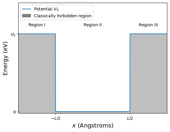
Fig. 2.21 The finite potential well of depth \(V_0\) and width \(L\), note the potential is \(V_0\) is the region \(x<-L/2\) and \(x>L/2\), and zero in the region \(-L/2\le x\le L/2\). The shaded gray area shows areas where a particle that has less energy than the potential would be classically forbidden. The unshaded areas are where a classical particle will be free to move.

2.6.2. The Schrödinger equation for a finite square well

Inside the finite square well, the region \(-L/2 \le x \le L/2\), the potential \(V(x)=0\) so the Schrödinger equation,

(2.14)\[ \frac{-\hbar^2}{2m}\frac{d^2\psi(x)}{d{x}^2}+V(x)\psi(x) =E\psi(x), \]

can be written as

(2.15)\[\begin{split} -\frac{\hbar^2}{2m}\frac{d^2\psi(x)}{d{x}^2}&=E\psi(x)\\ \frac{d^2\psi(x)}{d{x}^2}&=-\frac{2mE}{\hbar^2}\psi(x)\\ &=-k^2\psi(x). \end{split}\]

The last step is achieved by substituting equation (2.3) into equation (2.4). Solutions to this equations have the form

(2.16)\[\begin{split} \psi(x)=&A_1e^{ikx}+B_1e^{-ikx}\\ =&A\sin(kx)+B\cos(kx). \end{split}\]

I have provided two ways of writing the solution and as with the infinite square well we will use the form that makes the mathematic as simple as possible. This will turnout to be the triginometric form inside the well and the exponental form outside the well. This is the same as we saw in the step potential solutions and the infinite square well.

Outside the finite square well, the region \(-L/2 > x\) and \(L/2 < x\) the potential is \(V(x)=V_0\) so the Schrödinger equations can be written as

(2.17)\[\begin{split} -\frac{\hbar^2}{2m}\frac{d^2\psi(x)}{d{x}^2}+V_0\psi(x) &=E\psi(x)\\ \frac{d^2\psi(x)}{d{x}^2}&=-\frac{2m(E-V_0)}{\hbar^2}\psi(x)\\ &=-k^2\psi(x). \end{split}\]

Note that \(k\) will be different for each region of the potential well.

What happens when \(E<V_0\)? In this case the term \(E-V_0\) will be negative which makes \(k\) imaginary. Recall that \(k\) is written as:

(2.18)\[ k=\sqrt{\frac{2m(E-V_0)}{\hbar^2}}=\sqrt{-\frac{2m(V_0-E)}{\hbar^2}}=i\sqrt{\frac{2m(V_0-E)}{\hbar^2}} = i\beta. \]

The expression in the first square root will always be negative when \(E<V_0\) so we simplfy and express \(k\) as an imaginary number with a magnitude \(\beta\). If we substitute equation (2.18) into the general solution to the Schrodinger equation (2.16) we find

(2.19)\[ \psi(x)=A_2e^{ikx}+B_2e^{-ikx}=A_2e^{-\beta x}+B_2e^{\beta x} \]

You can now see that the same situation as we saw in the potential step problem happens again. The wave function that described the particle with energy \(E<V_0\) outside the box is an exponential function doesn’t have an imaginary argument, this describes a function that decays exponentially. Note, that even though the function outside the box does not oscillate it is still a function that descibes the state of a particle and therefore we still refer to it as a wavefunction.

Before we move on, here are some questions to consider:

• Q1: Can you test if equation (2.19) this is a solution to the Schrodinger equation?

• Q2: Given that \(\psi(x)\) must be finite, how would this constrain the solutions for \(x\rightarrow \pm\infty\)?

Answers

For question 1 you differentiate the function twice and substitute into equation (2.14).

\[\begin{split} \frac{d^2}{dx^2}\left( A_2e^{-\beta x}+B_2e^{\beta x} \right)=\beta^2 \left( A_2e^{-\beta x}+B_2e^{\beta x} \right)=\beta^2\psi(x)\\ \end{split}\]

Substitute into equation (2.14) and you obtain

\[\begin{split} -\frac{\hbar^2}{2m}\beta^2\psi(x)+V_0\psi(x)=E\psi(x)\\ \beta=\sqrt{-\frac{(2mE-V_0)}{\hbar^2}} \end{split}\]

which is what we found in equation (2.19)

In question 2 you are asked to consider how to make the wavefunction finite, i.e. \(|\psi(x)|^2\) must have a value when integrated overall all values of \(x\). We can do this by letting the wavefunction in regions I & III tend towards 0 as \(x\rightarrow\pm\infty\). If in region I, where \(x<-L/2\), we let \(A_2=0\) and in region III, where \(x>L/2\), \(B_2=0\) then this will occur and the function becomes finite. Don’t worry if you didn’t get this just yet we will now look at this in more detail.

2.6.3. The wavefunctions for a finite square well

Our potential well is composed of three regions and the particle will have an energy less than the potentail, i.e. \(E<V_0\). In order that the wavefunction can be normalised we make the following choices so that as \(x\rightarrow\pm\infty\) the value of \(\psi(x)\rightarrow 0\). We will also choose the trigonometic form of the wavefunction inside the potential, recall this is to make the maths easier.

\[\begin{split} &\text{Region I: } V(x) = V_0 ~~~~~~~~~~~~~~~~ x \leq-\frac{L}{2} ~~~~~ \psi_{I} = A e^{\beta x} \\ &\text{Region II: } V(x) = 0 ~~~ -\frac{L}{2} \leq x \leq\frac{L}{2} ~~~~~~~ \psi_{II} = B \cos(k x) + C \sin(k x)\\ &\text{Region III:} V(x) = V_0 ~~~~~~~~~~~~~~ x \geq \frac{L}{2} ~~~~~~~ \psi_{III} = D e^{-\beta x} \end{split}\]

Why do we check for continuity?

\(\psi^{'}\) needs to be continuous to guarantee the existence of \(\psi^{''}\), whose existence is required from the first postulate. \(\large{\frac{d^2}{dx^2}}\) is a component of the kinetic energy operator. If the wavefucntion doesn’t have a well-defined second derivative, then the kinetic energy would be undefined, which is not possible.

The wavefunction will be the sum of all three components so we make sure that the wavefunction and it’s first derivative are continuous at any boundary. We apply the following boundary conditions to achive this

\[ \psi_{I}\left(-\frac{L}{2}\right) = \psi_{II}\left(-\frac{L}{2}\right) \text{ and } \psi_{II}\left(\frac{L}{2}\right) = \psi_{III}\left(\frac{L}{2}\right). \]

\[ \psi^{'}_{I}\left(-\frac{L}{2}\right) = \psi^{'}_{II}\left(-\frac{L}{2}\right) \text{ and } \psi^{'}_{II}\left(\frac{L}{2}\right) = \psi^{'}_{III}\left(\frac{L}{2}\right) \]

note there are two conditions for each boundary so we will endup with 2 sets of 2 simultanious equations.

Finally, our potential is symmetric about \(x=0\) so our wavefunction will either be a maximum or zero at \(x=0\) so that the probability distribution is symmetric about \(x=0\). We will call these even for \(\psi(x)=\psi(x)\) and odd when \(\psi(x)=-\psi(-x)\).

Even solutions:

\[\begin{split} x \leq-\frac{L}{2}:& ~~~ \psi_{I}(x) = A e^{\beta x} \\ -\frac{L}{2} \leq x \leq\frac{L}{2}:& ~~~ \psi_{II}(x) = B \cos(k x) \\ x \geq \frac{L}{2}:& ~~~ \psi_{III}(x) = D e^{-\beta x} \end{split}\]

Why are they called even solutions?

These are called even solutions because the function \(\cos(kx)\) is even, i.e. it is symmetric about \(x=0\). However, they will correspond to the odd values of \(n\). It is perhaps easier to see this by looking at plots of the wavefunctions in figure figure 2.23.

After imposing the boundary conditions we reach the following relation:

(2.20)\[ \beta = k\tan\left(k\frac{L}{2}\right)\Rightarrow \sqrt{V_o-E} = \sqrt{E}\tan\left(\frac{L\sqrt{2mE}}{2\hbar}\right) \]

Odd solutions:

\[\begin{split} x \leq-\frac{L}{2}: & ~~~ \psi_{I}(x) = -A e^{\beta x} \\ -\frac{L}{2} \leq x \leq\frac{L}{2}: & ~~~ \psi_{II}(x) = C \sin(k x) \\ x \geq \frac{L}{2}: & ~~~ \psi_{III}(x) = D e^{-\beta x} \end{split}\]

Why are they called odd solutions?

These are called odd solutions because the function \(\sin(kx)\) is odd, i.e. it is anti-symmetric about \(x=0\). However, they will correspond to the even values of \(n\). A bit confusion I know but the choice of \(n\) is arbitrary whilst the sine and cosine solutions are determined by the physics. It is perhaps easier to see this by looking at plots of the wavefunctions in figure figure 2.23.

After imposing the boundary conditions we reach the following relation:

(2.21)\[ \beta = -\frac{k}{\tan\left(k\frac{L}{2}\right)} \Rightarrow \sqrt{V_o-E} = -\frac{\sqrt{E}}{\tan\left(\frac{L\sqrt{2mE}}{2\hbar}\right)} \]

The actual solutions will be those corresponding to energies that obey equations (2.20) and (2.21). Once we find the allowed energies, we can go back and obtain the wavefunctions with the proper coefficients.

2.6.4. Finding the energy eigen values graphically

Unfortunately, we cannot find the allowed energies analytically. That means we can not rearrange either of equations (2.20) and (2.21) to make \(E\) the subject. Instead we we have to chose either a graphically or numerically method. What doe that mean? We can graph the left and right hand side equations (2.20) and (2.21) seperately as a function of energy \(E\) and look for the intersection points which will correspond to the allowed energy values (the energy eigen values). Below I have plotted the functions for the odd and even wavefunctions using the Desmos graphing tool, you can adjust the potential \(V\) and the length \(L\), you can also click on the intercept points to determine the energy and value of the function.

Below the same has been performed in python, you may launch the inteactive session using the colab button below.

Fig. 2.22 (Left) The left and right hand sides of equations (2.20) and (2.21) plotted as a function of energy. Note that the right hand side of both equations is identical hence there are only three functions plotted. The intercepts correspond to the roots of the equation and are the energies of the states in the finite square well. (right) the energies of the states are plotted inside the potential well, note that there are now a finite number that as you would expect have energies lower the \(V_0\).

Why does the caption to figure 2.22 say we are finding the roots to equations (2.20) and (2.21)? By rearraning the equations we find the following

\[\begin{split} \sqrt{V_0-E}-\sqrt{E}\tan\left(\frac{L\sqrt{2mE}}{2\hbar}\right)=0\\ \sqrt{V_0-E}+\sqrt{E}\cot\left(\frac{L\sqrt{2mE}}{2\hbar}\right)=0 \end{split}\]

This is of course how you will have found the roots of a polynomial or trigonometic equation in the past, now it is just a bit more challenging and we need a computer to do the work for us.

Here are some question to think about:

• Q1: How does changing the width effect the number and energy of the states?

• Q2: How does changing the potential effect the number and energy of the states?

• Q3: Is the ground state described by an even or an odd wavefunction?

• Q4: What is the minimum number of states?

• Q5: Do the energy levels follow the same pattern as the infinite square well, i.e. \(E_n=E_1n^2\)?

2.6.5. Plots of the wavefunctions and prbability densities

Now we know the energy eigen values we can use these to find expressions for the wavefunctions and probability densities. This may help you understand some of the choices we made up to this point. Take a look at the figure and consider again the choice of the wavefunction in the region I and III, and why we broke up the wavefunction into odd and even functions inside the well.

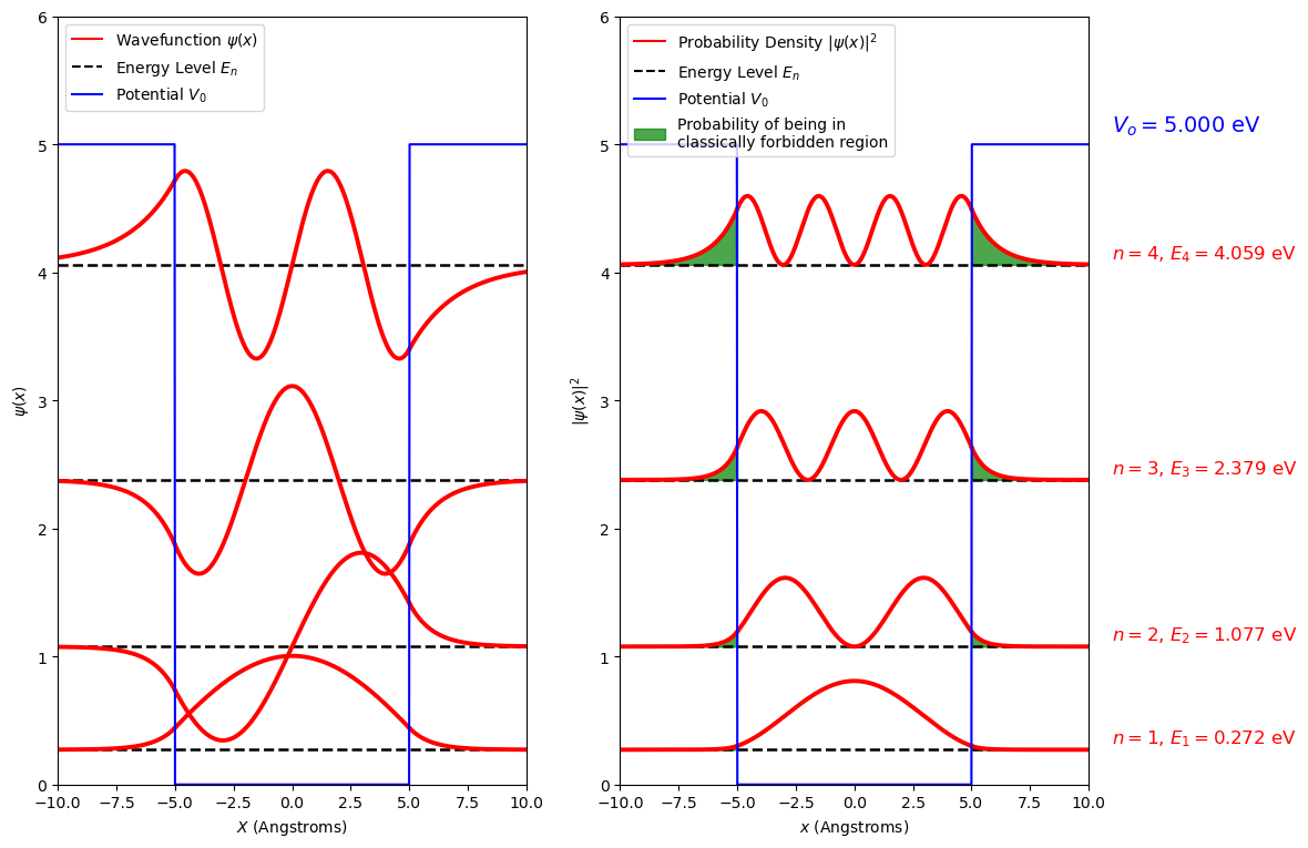
Fig. 2.23 A combined plot where the wavefunction (left) and probability density function (right) are plotted at the energy level of the state it represents. These are plotted to show values of \(x\) outside the well and in contrast to the infinite square well the wavefunction extends into these regions. On the (right) the probability of being outside the well is shown in green.

From these plots we can explain some of the behaviour of the energy levels as \(L\) and \(V_0\) are changed.

The first thing to note from the diagram above is that the wavefunction extend outside the potential, they enter what is sometime called the classically forbidden region. As with the potential step the quantum description of the particle allows it to tunnel into a region where the potential is larger than the energy of the particle. This is indicated by the shaded green area in the probability density plot. Note, this gets larger as the value \(V_0-E\) approaches zero.

The tunneling probability correspond to the area outside the box that has non-zero values of probability density. In the graphicaly representation, those areas are shaded in green. The integration of those areas provide the probability that the particle will tunnel outside the classically allowed region.

\[\begin{split} P\left(-\frac{L}{2}>x>\frac{L}{2}\right)=& \frac{\text{The area of the probability density that is shaded green}}{\text{The total area of the probability density}}\\ =&\large{\frac{\int^{\frac{-L}{2}}_{-\infty} |\psi(x)|^2\ dx +\int^{+\infty}_{\frac{L}{2}} |\psi(x)|^2\ dx }{\int_{-\infty}^{+\infty} |\psi(x)|^2\ dx }} \end{split}\]

where the denominator is 1 for a normalized wavefunction.

We can calculate \(P(-L/2>x>L/2)\), i.e. the size of the shaded green area, as a percentage of the total area:

The tunneling probabilities are:
  State #  1 tunneling probability =  0.83%
  State #  2 tunneling probability =  3.55%
  State #  3 tunneling probability =  9.25%
  State #  4 tunneling probability = 23.30%

2.6.6. A comparison between the energies of an infinite and finte square well

These values show what we have already deduced, that the closer the state is to the top of the potential the easier it is to spread outside of the potential. How does this effect the energy levels? Lower in the potential the wavelength of the wavfunction is more closely related to the width of the potential than it is higher in the potential. Compare the same width potential for the infinite and finite square well below.

Fig. 2.24 (Left) The infinite square well enegies upto the hight of the finite square well (right) of the same width. (right) the enrgies of a finite squre well of width 10 angstroms and depth 5 eV. Both show the states of an electron confined to these wells.

Notice that at energies closer to zero the infinite and finite energies are closer. As the energy of the state gets closer to the top of the finite potential it is smaller in the finite well than the infinite well. Why? The higher energy states allow the wavefunction in the finite squre well to spread out so the wavelength will be longer in the finite square well compared to the infinite squre well. A longer wavelength corresponds to a smaller value of \(k\) (wavenumber) and hence a lower energy state.