1.1. The Photoelectric effect

1.1.1. Origin of the photoelectric effect equation

It is one of those occasional paradoxes of experimental physics that the experiment first used by Hertz to establish Maxwell’s theory for the propagation of electromagnetic (EM) waves was also the same experiment that demonstrated the particle properties of EM waves. It was noted by Hertz that the current caused by light incident on a metal plate was higher for ultraviolet light than say for visible light. Let’s first take a step back from this experiment and define the process that was observed by Hertz and eventually explained by Einstein.

In the photoelectric effect, light incident on the surface of a metal plate, will stimulate the release of electrons. These electrons are called photoelectrons when emitted by the photoelectric effect. They are not a special type of electron we simply used this name to indicate how the electrons were produced. How does this process occur? In a simple model of a metal there is a regular array of atoms, the potential around each atom follows the expected \(V\propto\frac{1}{r}\), V is proportional to 1 over r, relationship that you would expect from your study of electrostatic point charges. Figure 1.2 shows the potential for a single atom, 5 atoms in a row, and an approximation when there are many atoms, as you would expect in a simple picture of a metal. The potential is plotted on the y-axis and the position is plotted on the x-axis. We will stick with only one dimension to simplify the pictures and avoid too much irrelevant detail in the physics explanation, but the argument can be extended to three dimensions and you will study these ideas later in another quantum mechanics course and again in statistical physics). For now one dimension is sufficient for us to understand what is occurring.

The Fermi Surface

We may call the dashed redline in the figure the Fermi Surface. This is the maximum energy the electrons possess in the potential. It is more correct to say this is the energy at a temperature of 0K but the value changes only by a very small amount at typical room temperatures so we can neglect this detail. The Fermi Surface plays a key role in many aspects of physics, for example the evolution of stars and the behaviour of semi-conductors and conductors. You will learn more about this important concept later in your degree.

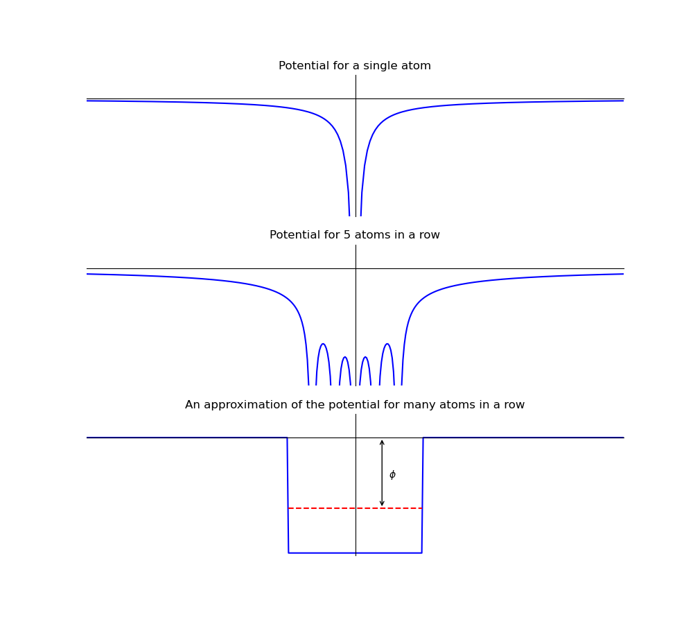
Fig. 1.2 The potentials for a single atom (upper), 5 atoms in a row (middle) and an approximation of the 5 atoms in a row (lower). The potential is plotted on the y-axis and the position is plotted on the x-axis. The red dashed line in the lower picture illustrates the typical upper limit of energy for electrons in the metal, many electrons will have an energy lower than this value.

To understand what figure 1.2 is showing consider that electrons with energy greater than zero are free from the metal (i.e. they can have any position value given on the x-axis). Those electrons with energy less than zero will be confined to the metal’s potential (i.e. they can only have position values that are between the vertical blue lines that represent the edge of the metal). The metal’s conduction electrons sit closer to the top of the potential, i.e. it will require the least amount of energy to release them from the metals potential, as indicated by the red dashed line in the figure 1.2. The minimum energy needed to release an electron from the metal’s potential is called the work function and given the symbol \(\phi\) (phi). A schematic representation of the process is shown in figure figure 1.3.

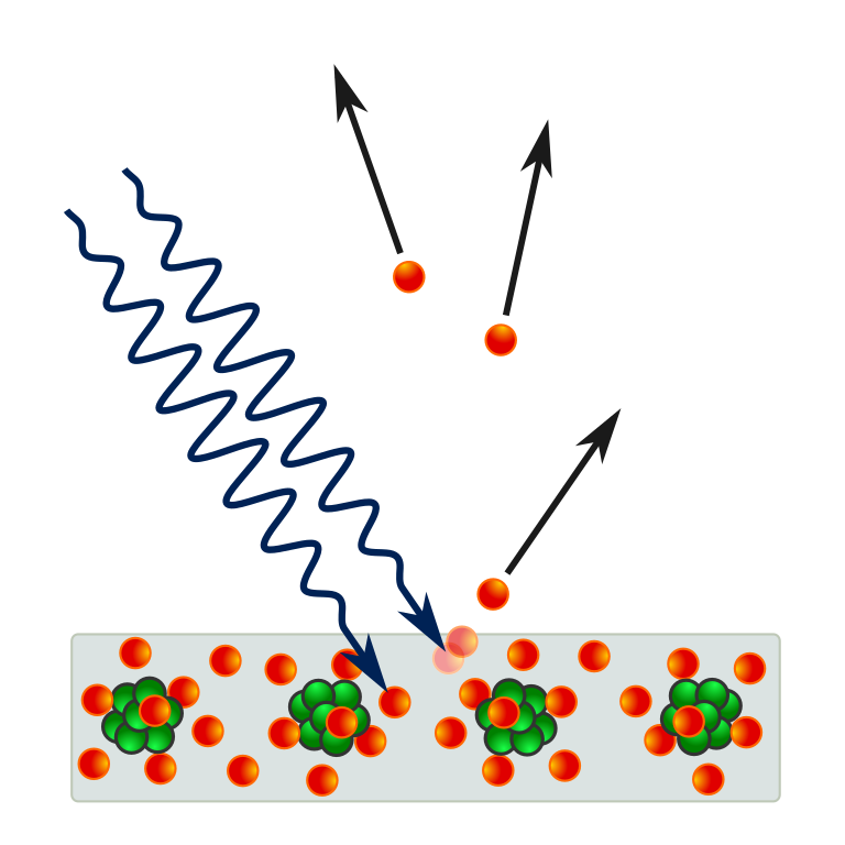
Fig. 1.3 A schematic illustration of the photoelectric effect in a solid [1].

For an incident photon with an energy \(E=hf\), the kinetic energy of the photoelectron after it escapes the metal is the energy that remains after doing work to escape the metal’s potential. It is given by the difference between the photon’s energy and the work function of the metal, this is expressed mathematically in equation (1.1).

(1.1)\[ \frac{1}{2}mv^2_\text{max}=hf-\phi. \]

Where \(m\) is the mass of the photoelectron, \(v_\text{max}\) is the maximum velocity of the emitted photoelectrons, \(h\) is Planck’s constant, \(f\) is the frequency of the incident photon, and \(\phi\) is the work function of the metal. Note that we calculate the maximum kinetic energy of the photoelectrons. We will discuss the reason for this shortly but first we must look at the experiment used to measure the photoelectric effect.

1.1.2. Applications: Sunrise on the moon!

There are many applications of the photoelectric effect, solar cells for example use a version of this physics to create electricity from incident photons. Instead of exciting the electrons out of the semiconductor used to make the solar cell the electrons are excited across the band gap of the semiconductor into the conduction band. My favourite application is to explain the sunrise on the moon that can be seen in figure 1.4 [2].

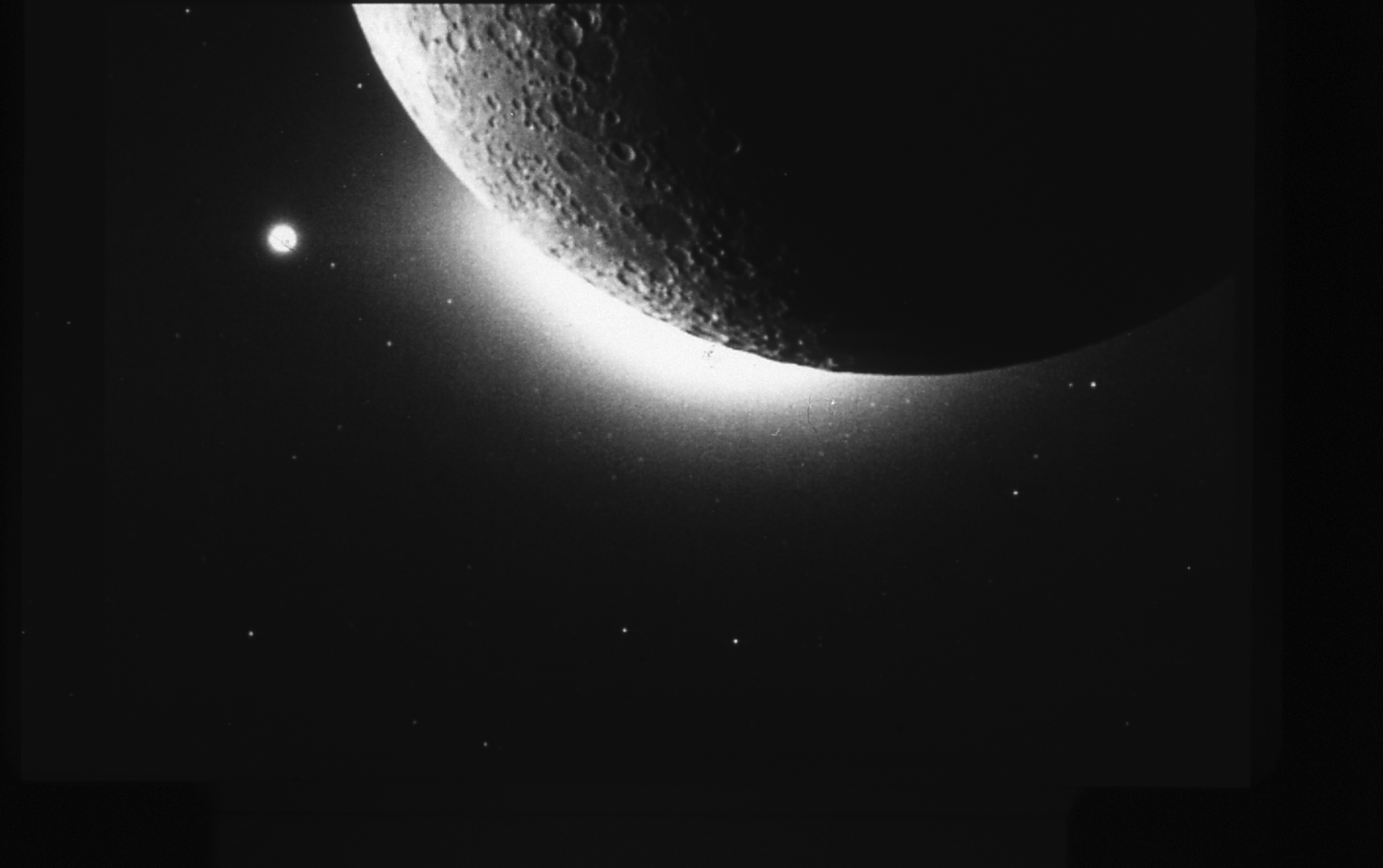
Fig. 1.4 A picture taken by the Clementine spacecraft of the Sun just about to rise over the moons horizon. On Earth scattering in the atmosphere is used to explain the observation of light before the sun has risen above the horizon. On the moon the very low density of particles just above the surface should prohibit this effect from occurring. (Credit: NASA).

The observation of light being scattered around the surface of the moon by jets of dust ejected from the surface of the moon is explained by the photoelectric effect. When the sunlight is incident of the surface of the moon the photoelectric effect charges the dust on the surface by exciting electrons out of the dust particles. The electrostatic force from the now charged dust particle can be used to explain the temporary atmosphere on the moon at the day-night terminator.

1.1.3. References:

[1] Ponor, CC BY-SA 4.0, via Wikimedia Commons

[2] Lunar dust transport by photoelectric charging at sunset.