1.4. Compton Scattering

1.4.1. Introduction

Compton scattering shows that the wavelength of an electromagnetic (EM) wave increases when it is scattered from an electron. The only way to explain this is to treat the incident EM was as a particle and apply the conservation of momentum. We will first review the experimental evidence then we will show that the change in the EM waves wavelength is modelled by treating the wave as a particle and applying the conservation of momentum. In Compton’s original experiment x-rays are scattered from a carbon target. The scattered x-rays are then passed into a Bragg spectrometer, on the left of figure 1.9, where the wavelength of the scattered x-ray is measured.

Fig. 1.9 Schematic diagram of Compton’s experiment. Compton scattering occurs in the graphite (carbon) target on the left. The slit passes X-ray photons scattered at a selected angle. The wave length of a scattered photon is measured using Bragg scattering in the crystal on the right in conjunction with ionization chamber.

1.4.2. Experimental Results

The data collected in the experiment showed that as the angle between the incident and scattered wave increases the wavelength of the scattered x-ray also increased. This is shown in figure 1.10 for scattering angles \(0^\circ\), \(45^\circ\), \(90^\circ\) and \(135^\circ\).

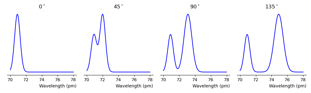
Fig. 1.10 A schematic representation of the Compton scattering data recorded by Arthur Compton.

At \(0^\circ\) only one peak is seen, with increased scattering angle this separates into two distinct peaks. The right peak is the Compton scattered x-ray from a loosely bound electron, it behaves similar to a free electron which is illustrated in figure 1.11. It is clear that the wavelength after scattering is larger than the wavelength of the incident x-rays.

Fig. 1.11 A schematic representation of Compton scattering. An x-ray is incident from the left of the figure on a stationary electron. The x-ray Compton scatters from the stationary electron, the process is inelastic and some energy is transferred from the x-ray to the electron. Hence, the energy of the electron increases and the energy of the x-ray photon decreases.

After scattering from a stationary electron the energy of an x-ray photon decreases. Hence, for an incident x-ray photon with wavelength \(\lambda\) the scattered x-ray photon will have longer wavelength denoted by \(\lambda^\prime\).

1.4.3. Theory

The Compton scattering formula is

(1.4)\[ \lambda^\prime-\lambda=\Delta\lambda=\frac{h}{mc}\left(1-\cos(\theta)\right). \]

Where \(\lambda^\prime\) is the wavelength of the scattered x ray photon, \(\lambda\) is the wavelength of the incident x ray photon, \(h\) is Planck’s constant, \(m\) is the mass of the scattered electron (note this can in practise be any particle but in this case it is an electron), \(c\) is the speed of light, and \(\theta\) is the scattering angle between the incident and the scattered photon.

Equation (1.4) is further evidence of the particle nature of EM radiation. It can be derived from the conservation of linear momentum (with a little application of relativity to account for the rest mass energy).

The left peak observed in each plot in figure 1.10 is the scattering from more tightly bound electrons. In contrast to the loosely bound electrons which scatter out of the carbon behaving similar to a free electron the more tightly bound electron remain bound to their carbon atom. In this case the mass \(m\) in equation (1.4) is the mass of the atom which recoils hence the shift in the observed wavelength is \(10^{-5}\) small due to the increased mass.

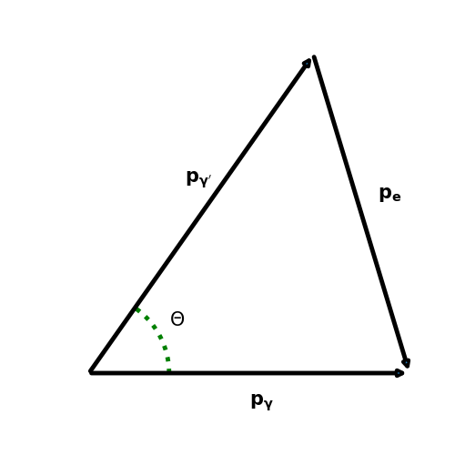
Fig. 1.12 The vector representation of electron and photons momentum in a Compton scattering event. The incident photon has momentum \(p_{\gamma}\), the scattered photon has momentum \(p_{\gamma^\prime}\), and the scattered electron has momentum \(p_e\). Note that the initial momentum of the electron is zero hence does not contribute.

A note about derivations

I will derive some but not all formula in this course. I will limit these derivations to examples where it illustrating something instructive about the physics we are studying. In this case, we are applying the conservation of momentum to a photon which illustrates that photons have particle like properties. This is reinforced by the excellent agreement between experiment and theory. You should avoid trying to memorise derivations, instead look at the physics applied to arrive at the solution. Try to break the derivation down into a set of very general steps and learn these, in this way you will be able to apply this knowledge to very different problems than the ones studied in class. Now, try applying equation (1.4) to the data provided in figure 1.10 to confirm the agreement with experimental results.

To derive equation (1.4) start by considering the conservation of momentum. From the diagram in figure 1.12 the vector addition gives

\[ \vec{\mathbf{p}_\gamma}=\vec{\mathbf{p}_{\gamma^\prime}}+\vec{\mathbf{p}_e} \]

\[ \vec{\mathbf{p}_e}=\vec{\mathbf{p}_{\gamma}}-\vec{\mathbf{p}_{\gamma^\prime}} \]

(1.5)\[ p_e^2=p_\gamma^2+p_{\gamma^\prime}^2-2p_\gamma p_{\gamma^\prime}\cos(\theta). \]

Where the last step was achieved using the cosine rule and the \(p\)’s are now the magnitudes of the vectors rather than vectors.

Next we consider the conservation of energy. To perform this step we need to consider the possibility that the electron will recoil at a very large velocity. Instead of simply considering the kinetic energy we will consider the full relativistic energy given by

(1.6)\[ E^2=p^2c^2+m^2c^4 \]

where \(E\) is the total energy, \(p\) is the momentum, \(m\) is the mass (in relativity you will later learn this is called the rest mass, for now just think of this as the mass and use the values you are familiar with, e.g. \(9.11\times10^{-31}\)kg for an electron) and of course \(c\) is the speed of light. Before the x-ray photon scatters from the electron the momentum is zero so the equation reduces to \(E=mc^2\), which you should be familiar with from your A-level physics course, after scattering it will have gained some momentum and we will denote the energy as \(E_e\). The energy of the photon before scattering we will give as \(E_\gamma\) and after as \(E_{\gamma\prime}\). The conservation of energy gives

(1.7)\[ E_\gamma+mc^2=E_{\gamma^\prime}+E_e \]

Which we can interpret as the sum of the energies before the scattering is equal to the sum of the energies after the scattering. Rearranging the equation for energy (1.6) to make the momentum of the electron the subject gives.

(1.8)\[ p_e^2c^2=E_e^2-m^2c^4 \]

Substitute (1.7) into (1.8) we obtain

(1.9)\[\begin{split} p_e^2c^2&=(E_\gamma-E_{\gamma^\prime}+mc^2)^2-m^2c^4 \\ &=E^2_\gamma-E^2_{\gamma^\prime}+m^2c^4 +2(E_\gamma -E_{\gamma^\prime})mc^2 -2E_\gamma E_{\gamma^\prime}-m^2c^4 \\ &=E^2_\gamma-E^2_{\gamma^\prime} +2(E_\gamma -E_{\gamma^\prime})mc^2 -2E_\gamma E_{\gamma^\prime} \end{split}\]

Multiply equation (1.5) by \(c^2\) and equating to equation (1.9) gives

\[ c^2p_\gamma^2+c^2p_{\gamma^\prime}^2-2c^2p_\gamma p_{\gamma^\prime}\cos(\theta) = E^2_\gamma-E^2_{\gamma^\prime} +2(E_\gamma -E_{\gamma^\prime})mc^2 -2E_\gamma E_{\gamma^\prime} \]

Using the relationship between a photons energy and momentum \(E=pc\) we can simplify the above equation to

(1.10)\[ E_\gamma-E_{\gamma^\prime}=\frac{E_\gamma E_{\gamma^\prime}}{mc^2}(1-\cos(\theta)) \]

Equation (1.4), the Compton scattering equation, can be obtained from equation (1.10) by substitution of \(E=\frac{hc}{\lambda}\).

I will leave is as an exercise for you to determine a similar relationship for the scattering angle of the electron relative to the scatteing angle of the photon.