1.8. Experimental evidence for electron structure#
The Bohr model predicts that electrons occupy orbits with specific energies. We will discuss two sources of experimental evidence that shows this is the correct interpretation.
The Franck-Hertz experiment.
Electron emission spectra.
1.8.1. The Franck-Hertz experiment#
A schematic picture of the Franck-Hertz experiment is shown in figure 1.21. In the Franck-Hertz experiment electrons are accelerated from a cathode (C) to an anode grid (G) and collected at (A). The current created by these accelerated electrons is recorded using an ammeter as indicated in the circuit. The tube through which the electrons are accelerated is filled with a low pressure gas.
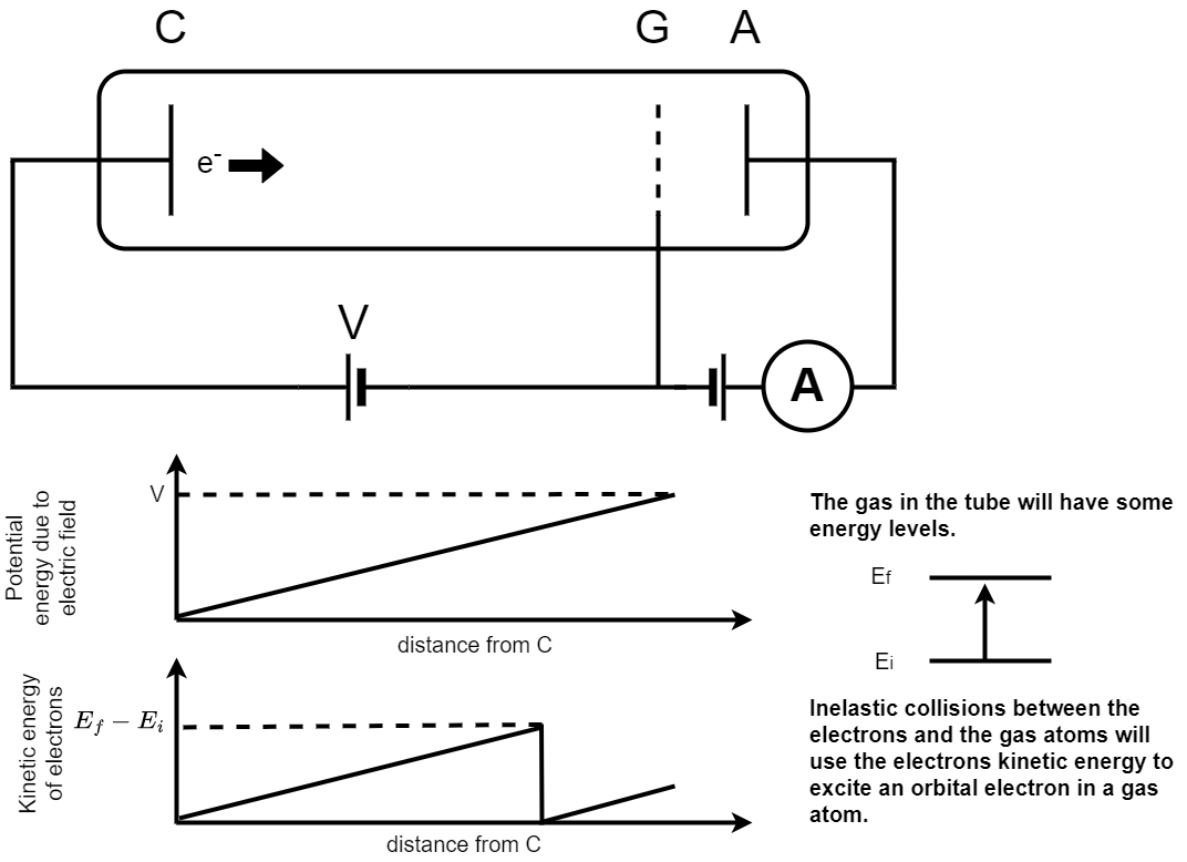
Fig. 1.21 A schematic picture of the Franck-Hertz experiment. In the Franck-Hertz experiment electrons are accelerated from a cathode (C) to an anode grid (G) and collected at (A). The current created by these accelerated electrons is recorded using an ammeter as indicated in the circuit. The tube through which the electrons are accelerated is filled with a low pressure gas. The two graphs show the accelerating potential as a function of the distance from the cathode (upper) and the velocity of the electrons as a function of distance from the cathode (lower). A schematic showing the initial and final energy level is given to the right of the figure.#
The accelerating potential between points C and G increases uniformly with distance from the cathode. The electrons will be subject to a constant accelerating force hence their kinetic energy will increase uniformly as they pass through the gas. Collisions between the electrons and the gas atoms can be either
Elastic, where the electrons kinetic energy does not change,
Inelastic, where the gas atoms gain some of the electrons kinetic energy.
When the accelerated electrons have gained kinetic energy equivalent to the difference between the ground state of the gas atom and an excited state they can scatter inelastically. This excites the orbital electrons in a gas atom to an excited state and reduces the energy of the accelerated electron to zero. They can then accelerate again until they pass through the grid at G.
The results of the Franck-Hertz experiment are shown in figure 1.22.
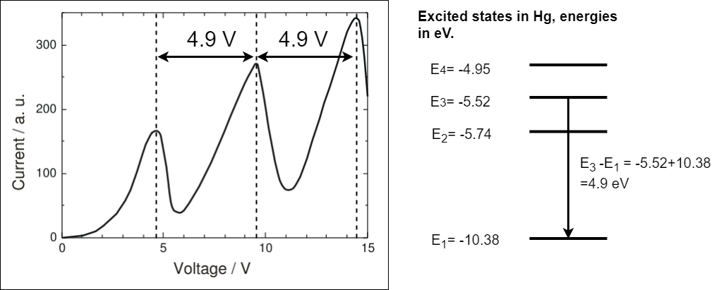
Fig. 1.22 A recreation of the results of the original Franck-Hertz experiment. The accelerating voltage is given on the x-axis and the current collected at A is given on the y-axis. The current rises to a maximum at about 4.9V then drops almost to zero, it rises again to a second maximum at 9.8V then drops almost to zero, a final maximum is seen at 14.7V. In the experiment electrons are accelerate through mercury. The excited states in mercury are given to the right of the graph.The difference between \(E_3\) and \(E_1\) is equal to the spacing between the observed maxima in the results.#
Why not the first excited state? (not for examination)
You may wonder why it is the second excited state and not the first that is observed. The cross section (i.e. probability of an interaction that excites this state) is much smaller than the for the second excited state. The reason is related to properties of the electron and properties of the electron states in mercury that are not included in the models you have studied so far. You will cover details like this in atomic and nuclear physics later in your degree.
As the accelerating voltage is increased the current rises to a maximum at about 4.9V then drops almost to zero, it rises again to a second maximum at 9.8V then drops almost to zero, a final maximum is seen at 14.7V. In the experiment electrons are accelerate through mercury. The excited states in mercury are given to the right of the graph. The difference between \(E_3=-5.52\) eV and \(E_1=-10.38\) eV is equal to the spacing between the observed maxima in the results hence the energy gained by an electron accelerated through 4.9 V. In class we will study the Neon example showing the same effect.
1.8.2. Atomic emission spectra#
A discharge lamp contains a low pressure gas and two electrodes. If the voltage is sufficiently high (100’s of volts) then the gas can ionise and when the electrons recombine with the atoms in the gas the de-excitation emits certain wavelengths of light. A spectrometer will allow us to see atomic emission spectra. The schematic representation of the hydrogen emission spectrum process is given in figure figure 1.23

Fig. 1.23 A schematic representation of the hydrogen transition lines. The principle quantum number is given for each orbital and the wavelength of emitted light is given next to the transition arrows. The series are named after scientists and grouped by a common quantum number for the final state of the decay. All Lyman series decay to the n=1 state, Balmer to the n=2, and Paschen to the n=3. You do not need to remember these names for assessment purposes.#
1.8.3. The Rydberg formula#
The Bohr model allows us to calculate the excited states of hydrogen-like atoms using equation (1.21)
This equation gives the energy in electron volts of the state with principle quantum number \(n\). An emission spectra shows the energy difference between two electron energy levels
where \(n_i\) is the principle quantum number of the initial state and \(n_f\) is the principle quantum number of the final state in the transition. \(Z\) is the number of protons in the nucleus, i.e. \(Zq_e\) is the charge of the nucleus.
We can convert to \(\lambda\) using \(E=\frac{hc}{\lambda}\)
Equation (1.22) is the Rydberg-Ritz formula and can be used to calculate the wavelength of emitted light given in figure 1.23. The quantity \(R=\frac{13.6Z^2}{hc}\) is called the Rydberg constant. Note that we stated with and equation that calculated energy in electron volts, the 13.6 has units of eV and so to get the correct unit of m for the wavelength we must either use \(h=4.14\times 10^{-15}\) eV s or convert 13.6 eV to Joules then use \(h=6.63\times 10^{-34}\) J s. In the next calculation we will take the second approach. For hydrogen this is
For hydrogen this has been measured as \(1.096\times10^{7}m^{-1}\).