The quantum harmonic oscillator

2.7. The quantum harmonic oscillator#

Particles oscillating in a solid can be employed as a simple model that described heat. You have already studied such oscillations in the Vibrations and Waves part of the course. In the classical case an object oscillated with harmonic motion if it is subjected to a restoring force that is proportional to the objects displacement and in the opposite direction. Mathematically we express this as

(2.22)#

F = - k^{^{'}} x .

We will use $k^{^{'}}$ as the constant of proportionality to differentiate it from the wavenumber $k = 2 π / λ$ used in the earlier lectures. You may be more familiar with the term ‘spring constant’ or ‘force constant’ for the constant of proportionality, as an object oscillating on a spring is the first harmonic oscillator you study. As with the other systems, e.g. the infinite and finite square wells, we will continue to work with energy and potentials rather than forces. We can calculate the potential, although you may already know the solution, by recalling that

F = - \frac{d U}{d x} .

So we can obtain an expression for U(x) by integration the expression for $F$ with respect to $x$ .

U (x) = - \int - k^{^{'}} x d x = k \frac{x^{2}}{2} + C

The condition that $U (0) = 0$ means that $C = 0$ and so we can ignore the constant of integration. A plot of the potential is shown in figure 2.25.

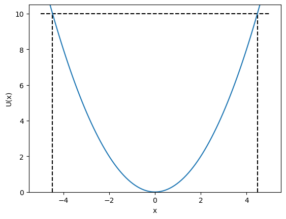
../_images/ae092882c50550f8cbed50394da581e69aef20fbeeb576af7f4e1553d111d9a4.png

A plot of the potential for the classical harmonic oscillator. The potential, U x, is plotted on the y axis the position of the oscillator from the average is plotted on the x axis. The potential is a parabola with the minimum a x equal 0. — Fig. 2.25 The classical harmonic oscillator potential, for a spring with $k^{^{'}} = 1$ . The horizontal line at $U (x) = 10$ J is the total energy, the maximum and minimum displacement are indicated by the vertical lines.#

In a classical system a particle of mass $m$ subject to a force given in equation (2.22) would oscillate with a sinusoidal motion and have an angular frequency of

ω = \sqrt{\frac{k^{^{'}}}{m}} .

The total energy of a particle oscillating with an amplitude $A$ would be

E = \frac{1}{2} k^{^{'}} A^{2} .

This quantity is illustrated in figure figure 2.25 by the horizontal dashed line at $10$ J.

We are interested in the behaviour of particles oscillating in a similar way. From our study of the infinite and finite square wells we already know that confining a particle to a potential leads of a set of discrete energy eigen states, i.e. whenever we measure the energy of the system it will correspond to the properties of a particle in one of these values. We know that in order to determine the energy eigen values we need a potential, an appropriate wave function and to then solve the time independent Schrodinger equation. The potential we already know from the classical harmonic oscillator.

(2.23)#

V (x) = \frac{1}{2} k^{^{'}} x^{2} = \frac{1}{2} m ω^{2} x^{2}

The choice of wavefunctions are more challenging and we will not prove what these are in this course I will provide them and you will learn the details at a later date. Recall from the properties of the wavefunction that it must be normalisable. For this to be the case the function we choose must approach zero as x approaches infinity.

| x | \to \pm \infty; ψ (x) \to 0

A gaussian function is a good example of a function with a peak at $x = 0$ and that falls to $0$ at $x \to \pm \infty$ and we will choose this for the lowest energy states. The eigen function for the first 3 states we choose will be

Quantum Number	Eigen function
0	$ψ_{0} (x) = A_{0} e^{- \frac{u}{2} x^{2}}$
1	$ψ_{1} (x) = A_{1} u^{\frac{1}{2}} x e^{- \frac{u}{2} x^{2}}$
2	$ψ_{2} (x) = A_{2} (1 - 2 u x^{2}) e^{- \frac{u}{2} x^{2}}$

where

u = \frac{(m k^{^{'}})^{1 / 2}}{ℏ} = \frac{m ω}{ℏ}

Note that unlike the Bohr model and he infinite square well we start the quantum numbers at zero. There is nothing deep to understand here it turn out to be mathematically convenient. Notice that in each case there is a polynomial function, known as the Hermite Polynomials, multiplied by a Gaussian function. The Hermite polynomials cause the eigen function to oscillate within the potential well and the Gaussian ensures that the above boundary conditions on $x$ are met. The Schrodinger wave equation for this system is then found by substituting in the correct potential

- \frac{ℏ^{2}}{2 m} \frac{d^{2} ψ}{d x^{2}} + \frac{1}{2} k^{^{'}} x^{2} ψ = E ψ

Substitute the eigen function into the Schrodinger equation and the pattern for the energy eigen values emerges. The $n = 0$ eigen function is substituted in as follows

\frac{d^{2}}{d x^{2}} [A_{0} e^{- \frac{u}{2} x^{2}}] = \frac{d}{d x} [A_{0} e^{- \frac{u}{2} x^{2}} (- u x)] = A_{0} e^{- \frac{u}{2} x^{2}} (- u x)^{2} + A_{0} e^{- \frac{u}{2} x^{2}} (- u) = ψ_{0} (u^{2} x^{2} - u)

Substituting into for $u$ and then into the Schrodinger equation quickly yields

E_{0} = \frac{1}{2} ℏ ω

Repeating this for the $n = 1$ and $n = 2$ states yields $E_{1} = \frac{3}{2} ℏ ω$ and $E_{2} = \frac{5}{2} ℏ ω$ . From this we can guess that the general solution for the energy eigen values of a harmonic oscillator potential are

E_{n} = (n + \frac{1}{2}) ℏ ω

These are plotted below for the first 6 states in an harmonic oscillator potential.

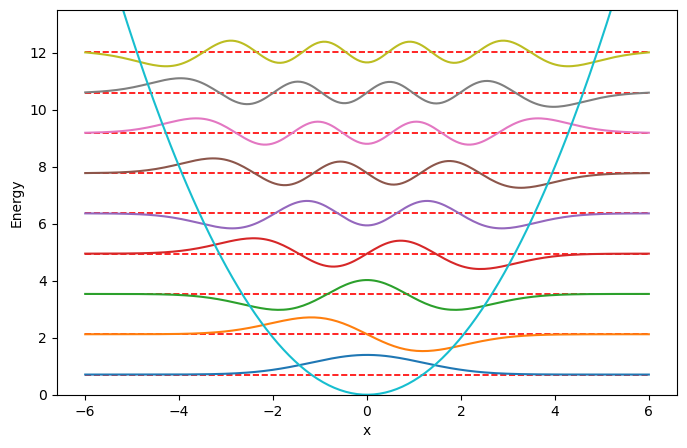
../_images/83746a268fa13b3f3dd6ebf0b3d0d287116be543c286ca3410e3dc16b6576982.png

A plot of the potential for the quantum harmonic oscillator. The potential, V x, is plotted on the y axis the position of the oscillator from the average is plotted on the x axis. The potential is a parabola with the minimum a x equal 0. The energy eigen values are shown as dashed red line at equally spaced intervals, the lowest has a value of energy greater than zero. The eigen functions are plotted ontop of the associated energy eigen value, these oscillate within the potential well and approach zero as as x tends towards plus and minus infinity. — Fig. 2.26 The quantum harmonic oscillator potential, for a spring with $k^{^{'}} = 1$ . The horizontal red lines at $E = (n + 1 / 2) ℏ ω$ eV are the energy eigen values for a particle confined to this potential. The energy eigen functions are plotted for each energy eigen value. This thing to note is that all of these functions approach zero as $x \to \pm \infty$ , i.e. they have a finite area and so can be normalised.#

There are two key results to keep in mind, the first turns out to be usefully in later courses, energy states are all equally spaced. The second point, if these energy states are a way to model heat and the lowest has an energy of $E_{0} = \frac{1}{2} ℏ ω$ then it is not possible to reach 0K, i.e. there will always be some vibrational energy in any system. This is called zero point energy.