1.2. The photoelectric effect experiment#
1.2.1. The Millikan Experiment#
A typical photoelectric effect experiment uses an evacuate glass vessel with an anode of work function \(\phi\) connected in series to a power supply and an ammeter. A schematic representation is given in figure 1.5. Light incident on the anode will allow photoelectrons to be emitted, the electric field between the anode and the cathode will accelerate the photoelectrons, collection at the cathode causes a current to flow that is recorded by the ammeter.
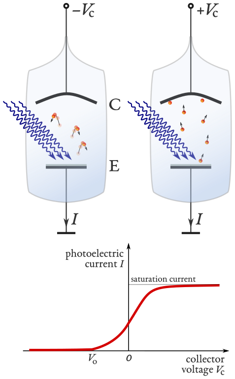
Fig. 1.5 A schematic representation of the photoelectric effect experiment. Light is incident on a metal plate (the anode labelled E) with sufficient energy for the metal to emit photoelectrons. A bias is applied between the metal plate (E) and a collector (the cathode labelled C) [1].#
In the left of figure 1.5 the bias is negative and creates an electric field pointing from E to C hence electrons are subjected to a force that reduces their velocity. If the bias is sufficiently large (with a magnitude greater than \(V_0\)) and with the correct polarity (direction) then the work done by the electric field will cause the photoelectrons lose all their kinetic energy before reaching C and return to E hence no current flows. In the right picture the bias is reversed and the electric field points from C to E. The photoelectrons are accelerated towards C and a current is observed. As the bias is increased above zero the electric field will
accelerate the electrons faster towards the collection anode and
allow the emission of electrons bound to the metal with a potential slightly greater than the incident photon energy.
Hence, an increase in current is observed which eventually saturates and becomes constant, as shown in the lower panel of figure 1.5.
1.2.2. Explanation of the experimental results#
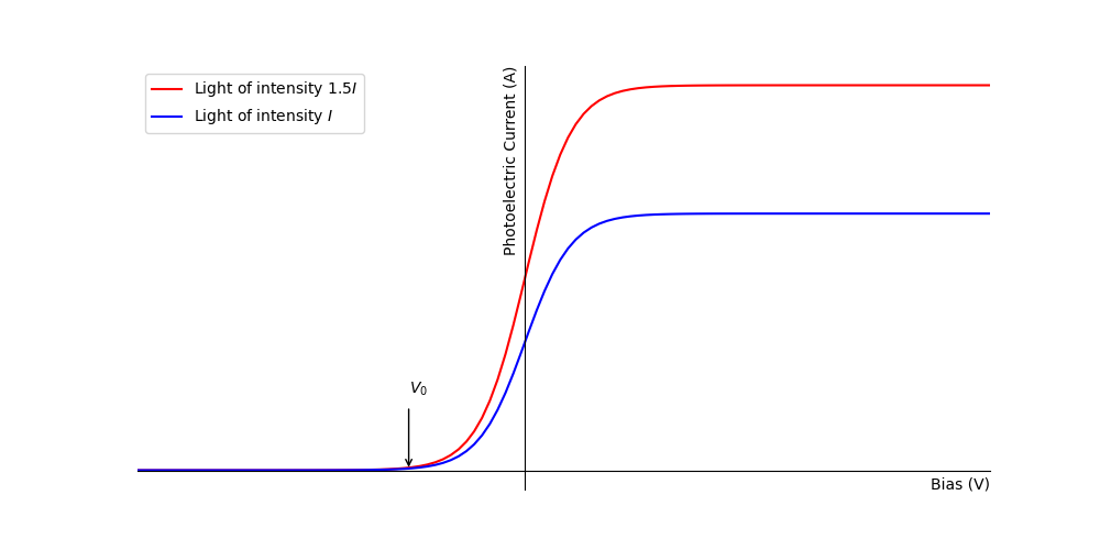
Fig. 1.6 A Schematic representation of the photoelectric current as a function of the bias. The blue line is for an arbitrary light intensity of \(I\) and the red line is for a light intensity of \(1.5I\).#
Note from figure figure 1.6is can be seen that the light intensity does not effect the value of the stopping potential \(V_0\), the potential at which the photoelectric current goes to zero. That the stopping voltage is independent of the light intensity is a consequence of the particle nature of light (and by extension EM radiation in general). A single incident photon can excite only one electron in the metal, hence there is a discrete amount of energy that each electron can receive from the incident light. This is in contrast to the wave nature in which a continuous distribution of energy from the EM wave might be expected to deliver any amount of energy to the metal given sufficient time. It is possible that two photons may interact with the same electron, however, this is very unlikely to occur and we may safely neglect this in our discussion.
The saturation current is also a consequence of the particle nature of light, for a given intensity of light there is a constant number of photons delivered per second. Hence, there is a maximum number of electrons that can be released for a given intensity, i.e. one photoelectron per photon. Beyond this value we can not increase the photocurrent by adjusting the bias (note: as mentioned above there is a small effect due to the electric field extending into the metal but this is negligible). Increasing the intensity of the light by 50% increases the the number of incident photons by 50% hence the saturation current increases by the same amount.
Equation (1.1) relates the maximum kinetic energy \(\frac{1}{2}mv^2_\text{max}\) of the photoelectrons to photon energy \(hf\) and the work function \(\phi\). The work done by the electric field \(W\) between C and E is given by \(W=qV\) where \(q\) is the charge of an electron and \(V\) is the stopping potential. When the stopping potential is \(V_0\) then the field does sufficient work to stop photoelectrons with an energy \(\frac{1}{2}mv^2_\text{max}\) hence we can rewrite equation (1.1) as
The stopping potential is plotted as a function of the frequency of the incident light in figure figure 1.7.
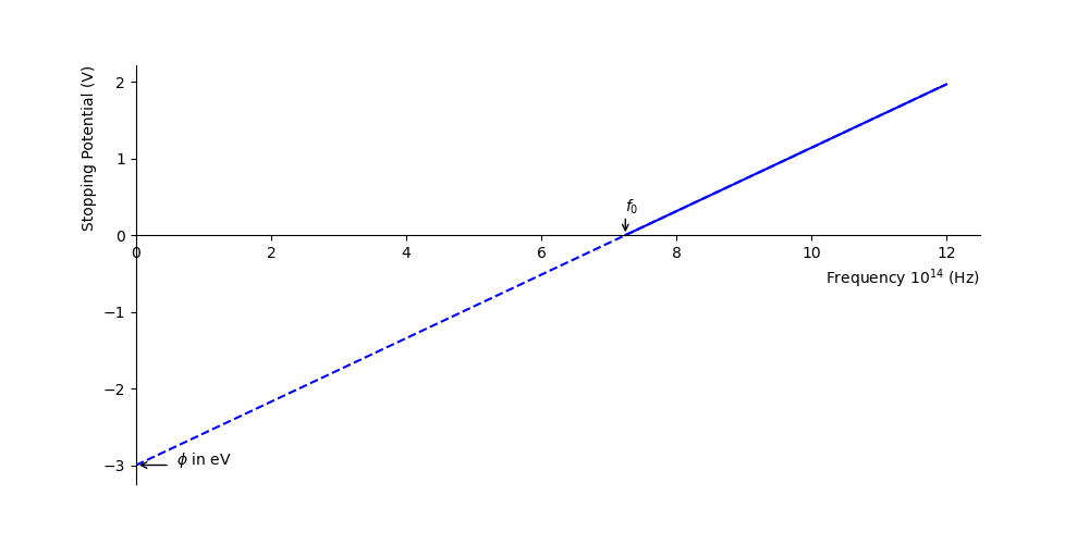
Fig. 1.7 The potential required to stop all photoelectrons \(V_0\) for a metal with a work function of \(\phi\)=3 eV. Marked on the x-axis is the threshold frequency \(f_0\). The dashed line below the threshold frequency is a linear extrapolation, the work function \(\phi\) is indicated on the stopping potential axis.#
You can use equation (1.2) to identify the work function \(\phi\) from the graph. How would you determine Planck’s constant from this experiment?
Planck’s constant can be determined from the gradient, rearranging equation (1.2) gives
Hence, multiplying the gradient by \(q\) will give you Planck’s constant. Note, that you can multiple the y-intercept (or indeed the gradient) by \(q=1.6\times10^{-19}\)C to find the workfunction in Joules (J) (for J.s for Planck’s constant) or by \(q=1\) to find the work function in eV.
1.2.3. References#
[1] Ponor, CC BY-SA 4.0, via Wikimedia Commons